ARGOS LOCATION
ARGOS ANIMAL TRACKING SYMPOSIUM ANNAPOLIS, MD MARCH 24-26, 2003 ... of successive frequency values received on board the satellite during the pass. ...

ARGOS LOCATION
E N D
Presentation Transcript
Slide 1: Roland Liaubet (CLS) liaubet@cls.fr Jean-Pierre Malard� (CLS) malarde@cls.fr
ARGOS LOCATION CALCULATION
Slide 2:Argos location principles Standard location processing description Others types of location Argos location class definition, interpretation and limits Argos location : main causes of error How to improve your number of locations and their accuracy Argos location software improvements foreseen
Summary
Slide 3:Argos location principles
Location based on Doppler shift measured on each message Apparent frequency shift observed when the receiver and the transmitter are in motion relative to each other
Slide 4:Doppler curve characteristics TCA/CTA definition
TCA Time of Closest Approach CTA Cross Track Angle Cross Track Angle Time of closest approach Doppler shift Time Sub-satellite track CTA TX Distance too short Distance too long TCA CTA also called distance from the ground sat track
Slide 5:Argos location principles
3 Hypothesis : Transmission frequency is stable during the satellite pass The platform is motionless during the satellite pass ( in principle) the altitude is known
Slide 6:Standard location processing
The location process follows 7 steps: A priori checks Geometric initialization Newton linearization Least-squares method Removing ambiguity Plausibility checks Location class estimation
Slide 7:Standard location processing
Standard location is attempted if at least 4 messages are received during a satellite pass 3 parameters are calculated : latitude, longitude, transmission frequency 1 : A priori checks
Slide 8:Standard location processing
TX frequency calculated from the previous satellite pass 2 messages -> 2 Doppler shifts -> 2 cones Intersection with ellipsoid = 2 positions Which is the true position? Which is the mirror position? 2 - Geometric initialization V1 V2
Slide 9:Standard location processing
Doppler equation Fr = g ( ?, ?,Fe ) is not a linear function regarding the 3 unknown parameters ?, ?,Fe Fr = g0+ ?g/? ? + ?g/?? + ?g/?Fe Fr = received frequency Fe = Transmission frequency Doppler shift = Fr - Fe 3 : Newton linearization
Slide 10:Standard location processing
4 : Least-squares method Location process consists in resolving by iteration the over-determined system ( nx3) made up of n Doppler equations : Fr = G(?, ?,Fe ) or A.X = Fr Where A is the matrix of the partial derivates of G with respect to ?, ?,Fe and, Fr the vector composed of successive frequency values received on board the satellite during the pass. A least squares method is used to determine the vector X by solving the normal system : ( At A ) X = At F The computation is performed twice using as initial values, results of the geometric initialization.
Slide 11:Standard location processing
4 : Least-squares method Fr Minimize the quantity : IC = SQRT (|| AX-F||2) = SQRT [ Sni=1( Fri � Fci)2 / (n-3)] The iterative processing stops when the residual error does not change significantly from an iteration to the next one IC = internal consistency or residual error
Satellite ground trackSlide 12:Standard location processing
5 : Removing ambiguity
Slide 13:Standard location processing
5 : Removing ambiguity How to choose the most probable solution 3 criterions : Smallest residual error Frequency continuity with respect to the last calculated frequency Minimum movement from the last calculated location
Slide 14:Standard location processing
6 : Plausibility checks The residual error of the chosen solution is significantly smaller than the one of the solution candidate The transmition frequency of the chosen solution is closer to the previous frequency than the one of the solution candidate Solution selected matches minimum distance traveled from the previous location Distance traveled from the previous location is compatible with the maximum velocity of the platform The position is delivered to the user if at least 2 out of 4 checks are successful.
Slide 15:Standard location processing
7 : Location class Locations classes provide information on the location process and an indication of the location accuracy. � There are four location classes: CLASS 0: estimated location error R > 1.500 m CLASS 1: estimated location error R < 1.500 m ( ~1000 m on each coordinate) CLASS 2: estimated location error R < 500 m ( ~ 350 m on each coordinate) CLASS 3: estimated location error R < 250 m ( ~ 150 m on each coordinate) R = Radius of the circle that should contain the actual position of the platform DISPOSE,TELEX or PUBLIC files contain only locations corresponding to classes requested by the user.
Slide 16:Radius error calculation
�Where : K : is the coefficient corresponding to the probability that the actual location of the transmitter is inside the circle with radius R. K = 1,414�corresponds to a probability of approximately 63% (*) HDOP : is the horizontal dilution of precision (*) Q : is the frequency noise estimator ( residual error) B : is the orbit error (B=100 m) (*) Argos location is assumed to be a bi-normal distribution The radius R of the circle of error is given by: (*) HDOP can be interpreted as the geometrical factor of observation error propagation
Slide 17:HDOP effect on location accuracy
At 8�, error = 1.414*200*0.25 ~ 70 m At 2�, error = 1.414*600*0.25 ~212 m TX closed to sat track TX at the horizon (2500km)
Slide 18:Effect of the PTT position relative to satellite ground track
Curves intersection is not precise Poor HDOP Curves intersection is optimal Good HDOP Curves intersection is not precise Poor HDOP
Slide 19:Classification limits
Residual error translates random errors Modeling errors or bias errors ( except for orbit error) are not taken into account in the ARGOS location and underestimated when calculating the radius of the circle of error
Slide 20:Two-message location processing
Only latitude and longitude are calculated. We assume the transmission frequency has not changed since the last location ( CLASS B) A priori checks Geometric initialization Removing ambiguity 1 criterion :minimum distance traveled from last location Plausibility checks 2 criteria : Solution selected matches minimum distance traveled from the previous location Distance traveled from the previous location is compatible with the maximum velocity of the platform
Slide 21:Two-message location
Location accuracy depends chiefly on the difference between the transmission frequency used in the geometric initialization and the actual PTT transmission frequency
Slide 22:Three message location
Latitude, longitude and transmission frequency are calculated. We assume the transmission frequency noise is negligible ( CLASS A) A priori checks Geometric initialization Newton linearization Resolution of a precisely determined linear system Removing ambiguity Frequency continuity with respect to the last calculated frequency Minimum distance traveled from last location Plausibility checks Transmitter frequency of the chosen solution is significantly closer to the previous calculated frequency than than the one of the solution candidate Minimum distance traveled from last location Distance traveled from the previous location is compatible with the maximum velocity of the platform
Slide 23:Standard location assuming a moving PTT
The platform is assumed to be moving from its previous location with a mean velocity in latitude and longitude ( and during the current satellite pass) Plast Pnew Standard locations only 0.5 h < delta T < 3.5 h The new location is kept if the residual error (IC) is smaller than the one obtained for a stationary platform
- Altitude - Speed Hardware TX power - ionosphere - troposphere - relativistic effect - timestamp - orbit error HardwareSlide 24:Argos location : main sources of error
- CTA
Slide 25:errors : effect on location accuracy
Frequency Drift Speed of the platform Error on altitude of the platform Ionosphere Effect Signal transmission power
Slide 26:Error caused by frequency drift ( due to temperature variation )
Doppler shift without freq. drift Measured Doppler shift Real position Computed position Drift
Slide 27:errors : USO quality
Slide 28:Error due to frequency drift
Error due to platform speed 400 m 7 km Elat(m) = 200*Vlat(km/h) Elon(m) = 100*Vlon(km/h)
Slide 29:Error of altitude
Error due to propagation in ionosphere 0.5 km 2.0 km
Slide 30:L��activit� solaire
Slide 31:Solar activity affects orbit precision
Slide 32:Impact of output power
PTT 18781 - CLASSES 1,2,3 - KL Nesdis data streams 0 10 20 30 40 50 60 70 80 90 100 0 250 500 750 1000 1250 1500 1750 2000 Distance from the true position (m) % 2W 0,25 W
Slide 33:Location performance
Slide 34:How to improve your locations
How to increase the number of messages received per satellite pass How to improve the location accuracy
Slide 35:Number of locations : Today, not enough messages received per satellite pass : it is the biggest cause of location problems Several explanations can be put forward : repetition rate too low, hardware quality and antenna efficiency, TX signal power too weak, TX environment (surrounding noise), data loss due to system occupancy ( TX concentration and transmission at the same frequency).
More location & better Precision
Slide 36:More locations & better Precision
How to increase the number of messages received and improve location accuracy Use multi-satellite service, Select good quality USO ( CLASS A recommended) Tuning TX parameters such as : output power, repetition rate, transmission frequency ( outside the Argos 1 band) Declare platform (average) altitude Declare correct maximum velocity of the platform
Slide 37:Current status PTT altitude is assumed to be known An error in PTT altitude is translated into an error varying between � and 4 times on longitude Command MOD is not much used Land platforms represent 20 % DEM : digital Elevation Model
Using a DEM in Argos location
Slide 38:USGS Model
30�� arc resolution / 100 m accuracy ( ? 1000 m)
Slide 39:Statistic in the European zone
Altitude error greater than 100 m in 40% Altitude declared at the User Office : 0 m in 93 % of cases
Slide 40:Validation
Experimentation Dh = 0m Dh = 1000m Using a DEM
Slide 41:Multi-pass location
Current status : Only single pass location Seven satellites in operation Waiting time between two successive satellite overpasses at 43 � latitude : 5 % : less than 5 minutes 25 % : less than 10 minutes 57 % : less than 15 minutes
Slide 42:Multi-pass location
Slide 43:Example
Slide 44:
Increase the number of standard locations Decrease the risk of selecting the wrong solution Advantages Multi-pass location Disadvantages When the TX is drifting too much When the platform is moving with a high speed