Download
1 / 10
100 likes | 708 Views
Separate classR, classV using midpoint of means ( mom ) method: calc a. a. vom V. vom R. d-line. d. v 2. v 1. std of these distances from origin along the d-line. FAUST Oblique (our best alg?) P R =P (X dot d)< a The forumula! 1 pass gives

E N D
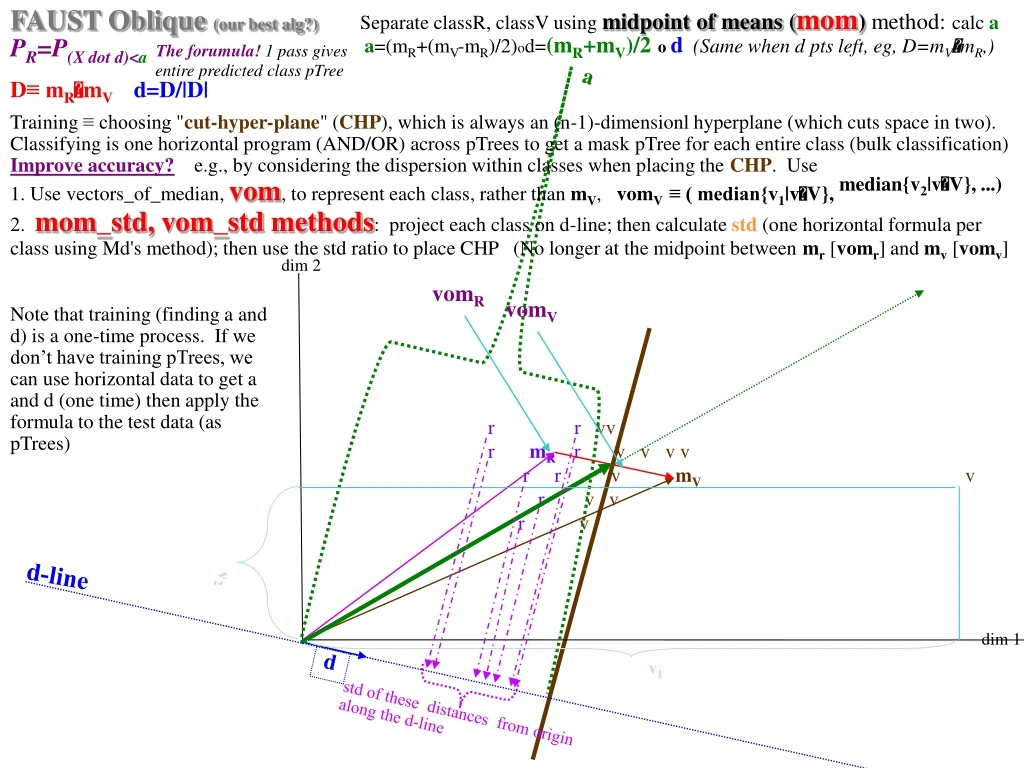
Separate classR, classV using midpoint of means (mom) method: calc a a vomV vomR d-line d v2 v1 std of these distances from origin along the d-line FAUST Oblique (our best alg?) PR=P(X dot d)<aThe forumula! 1 pass gives entire predicted class pTree D≡ mRmVd=D/|D| a=(mR+(mV-mR)/2)od=(mR+mV)/2o d(Same when d pts left, eg, D=mVmR,) Training ≡ choosing "cut-hyper-plane" (CHP), which is always an (n-1)-dimensionlhyperplane (which cuts space in two). Classifying is one horizontal program (AND/OR) across pTrees to get a mask pTree for each entire class (bulk classification) Improve accuracy? e.g., by considering the dispersion within classes when placing the CHP. Use 1. Use vectors_of_median, vom, to represent each class, rather thanmV, vomV≡ ( median{v1|vV}, 2. mom_std, vom_std methods: project each class on d-line; then calculate std (one horizontal formula per class using Md's method); then use the std ratio to place CHP (No longer at the midpoint between mr [vomr] and mv [vomv] median{v2|vV}, ...) dim 2 Note that training (finding a and d) is a one-time process. If we don’t have training pTrees, we can use horizontal data to get a and d (one time) then apply the formula to the test data (as pTrees) r r vv r mR r v v v v r r v mV v r v v r v dim 1
Mark S. said "Faust is fast... takes ~15 sec on the same dataset that takes over 9 hours with knn and 40 min with pTree knn. I’m ready to take on oblique, need better accuracy (still working on that with cut method ("best gap" method)." FAUST isthis manytimes faster than, Horizontal KNN2160taking 9.000 hours = 540.00 minutes = 32,400 sec. pCKNN: 160 taking .670 hours = 40.00 minutes = 2,400 sec. while Mdpt FAUST takes .004 hours = .25 minutes = 15 sec. "Doing experiments on faust to assess cutting off classification when gaps got too small (with an eye towards using knn or something from there). Results are pretty darn good… for faust this is still single gap, working on total gap (max of (min of prev and next gaps)) Here’s a new data sheet I’ve been working on focused on gov’t clients." Bill P: You might try tweaking BestClassAttributeGap-FAUST (BCAG FAUST) by using all gaps that meet a criteria (e.g., where the sum of the two stds from the two bounding classes add up to less than the gap width), Then just AND all of the mask pTrees. Also, Oblique FAUST is more accurate and faster as well. I will have Mohammad send what he has and please interact with him on quadratics - he will help you with the implementation. I wonder if in return we could get the datasets you are using for your performance analysis (with code of competitor algorithms etc.?) It would help us a lot in writing papers Mark S: I'm working on a number of benchmarks. Bill P: Maybe we can work together on Oblique FAUST performance analysis using your benchmarks. You'd be co-author. My students crunch numbers... Mark S: Vendor opp: Provides data mining solutions to telecom operators for call analysis, etc - using faust in an unsupervised mode - thots on that for anomaly detection. Bill P: FAUST should be great for that.
Multi-hop Data Mining (MDM): relationship1 (e.g., Buys= B(P,I) ties table1 Category color size wt store city state country 2 2 3 3 4 4 5 5 P 2 3 0 1 0 1 1 0 1 0 0 1 0 0 0 0 1 1 4 5 ct(|pAPpAND&iCPi)>mncf ct(|pAPp) friend of any in A will buy C if any in A buy C. ct(|pAPpAND |iCPi) >mncnf ct(|pAPp) Change to "a friend of any in A will buy something in C if any in A buy C. pc bc lc cc pe age ht wt (e.g., People=P=an axis with descriptive features columns) to table_2 (e.g., Items). Table2 (I=Items) is tied by relationship2 (e.g., Friends=F(P,P) ) to table3 (e.g., also P)... Can we do interesting clustering and/or classification on one of the tables using the relationships to define "close" or to define the other notions? P=People, I=Items, F(P,C)=Friends, B(C,I)=Buys Find all strong, AC, AP, CI frequent iff ct(PA)>minsup and confident iff ct(&pAPpAND &iCPi) > minconf ct(&pAPp) Says: "friend of all in A will buy C if all in A buy C." (AND always AND) closures: A freq then A+ freq. AC not conf, then AC- not conf I=Items F(P,P)=Friends 0 0 0 1 0 1 0 0 0 0 0 0 0 0 1 0 B(P,I)=Buys P=People Define the NearestNeighbor VoterSet of {f} using strong R-rules with F in the consequent? A correlation is a relationship A strong cluster based on several self-relationships (but different relationships, so it's not just strong implication both ways) is a set that strongly implies itself (or strongly implies itself after several hops (or when closing a loop). Dear Amal, Yes, we have looked at the 2012 cup too and you are right that it would form a good testbed for social media data mining work. Ya Zhu in our Sat gp is leading on "contests" and is looking at 2012 KDD Cup as well as Heritage Provider Network Health Prize (see kaggle.com). I am hoping also for a nice test bed involving the our Netflix datasets (which you and then Dr. Wettstein prepared as pTrees and all have worked on extensively - Matt Piehl and Tingda Lu particularly...). I am hoping to find (in the netflix contest related literature) a real-life social network (a social relationship between two copies of the netflix customers such as maybe, facebook friends, that we can use inconjunction with the netflix "rates" relationship between netflix customers and netflix movies. We would be able to do something with that set up (all as PTreeSet both ways).For those who are new to our little "group", Dr. Amal Shehan Perera is a senior professor in Sri Lanka and was (definitely a lead) researcher in our group for many years. He is the architect of using GAs to win the KDD Cup in both 2002 and 2006. He gets most of the credit for those wins, as it was definitely GA work in both cases that pushed us over the top (I believe anyway). He's the best!! You would be wise to stay in touch with him.Sat, Mar 24, Amal Shehan Perera <shehan@uom.lk: Just had a peek into the slides last week and saw a request for social media data. Just wanted to point out that the 2012 KDD Cup is on social media data. I have not had a chance to explore the data yet. If I do I will update you. Rgds,-amal
1 0 0 0 1 0 0 bpp 1 2 3 4 5 ... 3B 0 1 1 0 0 1 1 0 0 0 0 0 0 0 1 0 0 0 1 0 0 1 1 2 2 0 0 1 0 0 0 1 3 3 1 0 0 0 1 0 0 4 4 0 0 1 0 0 0 0 5 5 AHG(P,bpp) ... ... 7B 7B P P gene chromosome bpp 1 2 3 4 5 ... 3B pc bc lc cc pe age ht wt 1 0 0 0 1 0 0 0 1 1 0 0 1 1 0 0 0 0 0 0 0 1 0 0 0 1 0 0 0 0 1 0 0 0 1 1 0 0 0 1 0 0 0 0 1 0 0 0 0 AHG(P,bpp) Bioinformatics Data Mining: Most bioinformatics done so far is not really data mining but is more toward the database querying side. (e.g., a BLAST search). What would be real Bioinformatics Data Mining (BDM)? A radical approach View whole Human Genome as 4 binary relationships between People and base-pair-positions (ordered by chromosome first, then gene region?). AHG is the relationship between People and adenine (A) (1/0 for yes/no) THG is the relationship between People and thymine (T) (1/0 for yes/no) GHG is the relationship between People and guanine (G) (1/0 for yes/no) CHG is the relationship between People and cytosine (C) (1/0 for yes/no) Order bpp? By chromosome and by gene or region (level2 is chromosome, level1 is gene within chromosome.) Do it to facilitate cross-organism bioinformatics data mining? This is a comprehensive view of the human genome (plus other genomes). Create both a People-PTreeSet and PTreeSet vertical human genome DB with a human health records feature table associated with the people entity. Then use that as a training set for both classification and multi-hop ARM. A challenge would be to use some comprehensive decomposition (ordering of bpps) so that cross species genomic data mining would be facilitated. On the other hand, if we have separate PTreeSets for each chrmomsome (or even each regioin - gene, intron exon...) then we can may be able to dataming horizontally across the all of these vertical pTree databases. The red person features used to define classes. AHGp pTrees for data mining. We can look for similarity (near neighbors) in a particular chromosome, a particular gene sequence, of overall or anything else.
A facebook Member, m, purchases Item, x, tells all friends. Let's make everyone a friend of him/her self. Each friend responds back with the Items, y, she/he bought and liked. Facebook-Buys: I≡Items I≡Items I≡Items F≡Friends(M,M) Members F≡Friends(K,B) F≡Friends(K,B) Buddies Buddies 1 0 1 1 4 1 1 0 0 1 1 1 1 4 4 0 1 0 0 3 0 0 1 1 0 0 0 0 3 3 1 0 0 1 2 1 1 0 0 0 0 1 1 2 2 0 0 1 0 1 0 0 0 0 1 1 0 0 1 1 P≡Purchase(M,I) P≡Purchase(B,I) P≡Purchase(B,I) Kiddos Kiddos 2 4 4 4 2 2 3 3 3 3 3 3 2 2 4 4 2 4 1 5 5 5 1 1 Members Groupies Groupies 4 4 1 1 0 0 1 1 1 1 4 4 1 2 4 2 2 2 4 1 3 3 0 0 1 1 0 0 0 0 3 3 2 2 1 1 0 0 0 0 1 1 2 2 0 0 1 1 0 1 0 0 1 0 1 1 1 1 0 1 1 0 1 1 1 0 1 1 1 1 1 1 0 1 0 1 1 0 1 1 1 1 1 0 1 1 1 1 0 0 1 1 1 1 1 1 1 1 1 0 1 1 1 1 1 0 0 0 0 0 0 1 1 1 4 4 4 3 3 3 2 2 2 1 1 1 4 4 4 0 0 0 0 1 1 0 0 1 1 1 0 0 0 0 0 0 0 Others(G,K) Compatriots (G,K) 1 1 1 1 1 1 1 1 1 1 1 0 0 0 1 1 1 1 1 1 2 2 2 1 0 0 0 1 1 0 0 Kx=OR Ogx frequent if Kx large (tractable- one x at a time and OR. gORbPxFb XI MX≡&xXPx People that purchased everything in X. FX≡ORmMXFb = Friends of a MX person. So, X={x}, is Mx Purchases x strong" Mx=ORmPxFmx frequent if Mx large. This is a tractable calculation. Take one x at a time and do the OR. K2 = {1,2,4} P2 = {2,4} ct(K2) = 3 ct(K2&P2)/ct(K2) = 2/3 Mx=ORmPxFmx confident if Mx large. ct( Mx Px ) / ct(Mx) > minconf To mine X, start with X={x}. If not confident then no superset is. Closure: X={x.y} for x and y forming confident rules themselves.... ct(ORmPxFm & Px)/ct(ORmPxFm)>mncnf Fcbk buddy, b, purchases x, tells friends. Friend tells all friends. Strong purchase poss? Intersect rather than union (AND rather than OR). Ad to friends of friends K2={2,4} P2={2,4} ct(K2) = 2 ct(K2&P2)/ct(K2) = 2/2 K2={1,2,3,4} P2={2,4} ct(K2) = 4 ct(K2&P2)/ct(K2)=2/4
Multi-level pTrees for data tables: n-row table, row predicate (e.g., a bit slice pred, or a category map) and row ordering (e.g., asc on key; spatial data, col/row-raster, Z=Peano, Hilbert), sequence of pred truth bits (1/0) is raw or level-0predicate map (pMap) for table, pred, row order. gte75% str=5 pMC=red 0 0 1 gte50% str=5 pMC=red 0 0 1 pure1 str=5 pMC=red 0 0 0 gte25% str=5 pMC=red 1 1 1 0 1 1 1 0 1 0 1 0 0 level-2 gte50% stride=2 1 1 pMgte50%,s=4,SL,0 0 1 1 1 level-1 gt50 stride=4 pMap level-1 gt50 stride=2 pMap IRIS Table NameSLSWPLPWColor setosa 38 38 14 2 red setosa 50 38 15 2 blue setosa 50 34 16 2 red setosa 48 42 15 2 white setosa 50 34 12 2 blue versicolor 51 24 45 15 red versicolor 56 30 45 14 red versicolor 57 28 32 14 white versicolor 54 26 45 13 blue versicolor 57 30 42 12 white virginica 73 29 58 17 white virginica 64 26 51 22 red virginica 72 28 49 16 blue virginica 74 30 48 22 red virginica 67 26 50 19 red pred: rem(div(SL/2)/2)=1 order: given order gte50% stride=5 pMSL,1 1 0 0 pure1 str=5 pMSL,1 0 0 0 gte25% str=5 pMSL,1 1 1 1 gte75% str=5 pMSL,1 1 0 0 pMSL,0 0 0 0 0 0 1 0 1 1 1 1 0 0 0 1 pMColor=red 1 0 1 0 0 1 1 0 0 0 0 1 0 1 1 pMSL,1 1 1 1 0 1 1 0 0 1 0 0 0 0 1 1 predicate: remainder(SL/2)=1 order: the given table order pred: Color='red' order: given ord Raw pMap, pM, decomp to mutual excl, coll exh bit ints, bit-inte-pred, bip (e.g., pure1, pure0, gte50%One), bip stride=m level-1 pMap of pM is the string of bip truths gened by bip to consec ints of decomp. Decomp equiwidth, int seq is fully determined by width=m>1, AKA, stride=m gte50% stride=5 pMPW<7 1 0 0 pred: PW<7 order: given gte50% st=5 pMap predicts setosa. pMgte50%,s=4,SL,0≡ gte50% stride=4 pMSL,0 0 1 1 1 gte50% stride=8 pMSL,0 0 1 gte50% stride=4 pMSL,0 0 1 1 1 rem(SL/2)=1 ord: given pred: rem(SL/2)=1 ord: given order pM all its lev1 pMaps=pTree of same name as pM pMPW<7 1 1 1 1 1 0 0 0 0 0 0 0 0 0 0 pMSL,0 0 0 0 0 0 1 0 1 1 1 1 0 0 0 1 1 pMSL,0 0 0 0 0 0 1 0 1 1 1 1 0 0 0 1 1 gte50%; es=4,8,16; SL,0 pTree: R11 1 0 0 0 1 0 1 1 pTgte50%_s=4,8,16_SL,0 lev2 pMap= lev1 pMap on a lev1. (1col tbl) raw level-0 pMap gte50_pTrees11 1 gte50% stride=16 pMSL,0 0
gte50 Satlog-Landsat stride=64, classes: redsoil cotton greysoil dampgreysoil stubble verydampgreysoil R G ir1 ir2 class WL band 1 [w1,w2) w1 w1 2 w2 w2 [w2,w3) ... [w3,w4) ... ... 4436 [w4,w5) w5000 w5000 WLs WLs pixels WLs 21 43 110 160 3 18 21 21 21 21 43 43 43 43 110 110 110 110 0 0 0 0 0 0 2 1 1 1 1 1 ... ... ... ... ... ... 255 255 255 255 255 255 202 14 0 160 160 160 160 3 3 3 3 18 18 18 18 r r r r c c c c g g g g d d d d s s s s v v v v 29 152 230 cl cl cl cl 202 202 202 202 14 14 14 14 0 0 0 0 1 1 1 1 0 0 0 0 0 0 0 0 10 0 0 10 0 0 0 0 1 10 10 0 10 0 0 0 0 0 1 29 29 29 29 152 152 152 152 230 230 230 230 0 0 0 0 0 0 0 0 0 0 0 0 0 78 4 78 78 78 0 1 4 78 1 0 0 1 0 1 0 0 0 0 0 0 0 0 0 0 0 0 0 0 0 155 0 1 7 1 0 155 155 155 155 1 0 0 0 0 7 0 1 0 0 0 0 0 0 0 0 0 0 0 0 0 0 0 2 0 0 54 0 0 0 54 54 54 0 54 0 0 2 0 0 Rclass ir2class Gclass ir1class ir2 G ir1 ir2 ir1 ir2 class Given a relationship, it generates 2 dual tables 0 0 0 0 0 0 1 0 0 0 0 0 0 0 0 0 0 0 0 0 0 0 0 0 0 0 0 0 1 1 0 1 1 0 1 0 1 0 0 w1 1 2 w2 1 2 1 1 1 1 1 1 2 1 2 2 1 0 0 0 0 0 1 0 0 0 0 0 0 0 1 0 0 0 0 0 0 1 0 0 0 ... ... ... ... ... ... ... ... ... ... ... ... ... ... ... ... 0 1 1 1 0 0 0 1 1 0 0 0 1 1 0 1 0 0 1 0 0 0 1 0 4436 4436 w5000 255 4436 255 255 255 255 4436 255 4436 255 255 255 255 1 0 0 1 0 0 0 0 0 1 1 1 0 1 0 0 0 0 0 1 0 0 0 0 R G G pixels pixels R ir1 ir2 pixels ir1 R G R WLs pixels pixels Gir1 Rir2 Rir1 Gir2 RG ir1ir2 gte50 Satlog-Landsat stride=320, get: 320-bit strides start end cls cls 320 strd 2 1073 1 1 2 321 1074 1552 2 1 322 641 1553 2513 3 1 642 961 2514 2928 4 2 1074 1393 2929 3398 5 3 1553 1872 3399 4435 _7 3 1873 2192 4436 3 2193 2512 4 2514 2833 5 2929 3248 7 3399 3718 7 3719 4038 7 4039 4358 Note: stride=320, means are way off and will produce inaccurate classification.. lev0 pVector is a bit string w 1bit/rec. lev1 pVector=bit string wbit/rec/stride, =pred_truth applied to record stride. levN pTree = levK pVec (K=0...N-1) all with same predicate and s.t each levK stride contained within 1 levK-1 stride. R G ir1 ir2 cls means stds means stds means stds means stds 1 64.33 6.80 104.33 3.77 112.67 0.94 100.00 16.31 2 46.00 0.00 35.00 0.00 98.00 0.00 66.00 0.00 3 89.33 1.89 101.67 3.77 101.33 3.77 85.33 3.77 4 78.00 0.00 91.00 0.00 96.00 0.00 78.00 0.00 5 57.00 0.00 53.00 0.00 66.00 0.00 57.00 0.00 7 67.67 1.70 76.33 1.89 74.00 0.00 67.67 1.70 The table is (and it generates the [labeled by value] relationships):
R G ir1 ir2 std 8 15 13 9 1 8 13 13 19 2 5 7 7 6 3 6 8 8 7 4 6 12 13 13 5 5 8 9 7 7 R G ir1 ir2 mn 62.83 95.29 108.12 89.50 1 48.84 39.91 113.89 118.31 2 87.48 105.50 110.60 87.46 3 77.41 90.94 95.61 75.35 4 59.59 62.27 83.02 69.95 5 69.01 77.42 81.59 64.13 7 FAUST Satlog evaluation 1 2 3 4 5 7 tot 461 224 397 211 237 470 2000 TP actual 99 193 325 130 151 257 1155 TP nonOb L0 pure1 212 183 314 103 157 330 1037 TP nonOblique 14 1 42 103 36 189 385 FP level-1 50% 322 199 344 145 174 353 1537 TP Obl level-0 28 3 80 171 107 74 463 FP MeansMidPoint 359 205 332 144 175 324 1539 TP Obl level-0 29 18 47 156 131 58 439 FP s1/(s1+s2) 410 212 277 179 199 324 1601 TP 2s1/(2s1+s2) 114 40 113 259 235 58 819 FP Ob L0 no elim 309 212 277 154 163 248 1363 TP 2s1/(2s1+s2) 22 40 65 211 196 27 561 FP Ob L0 234571 329 189 277 154 164 307 1420 TP 2s1/(2s1+s2) 25 1 113 211 121 33 504 FP Ob L0 347512 355 189 277 154 164 307 1446 TP 2s1/(2s1+s2) 37 18 14 259 121 33 482 FPOb L0425713 2 33 56 58 6 18 173 TP BandClass rule 0 0 24 46 0 193 263 FP mining (below) red green ir1 ir2 abv below abv below abv below abv below avg 1 4.33 2.10 5.29 2.16 1.68 8.09 13.11 0.94 4.71 2 1.30 1.12 6.07 0.94 2.36 3 1.09 2.16 8.09 6.07 1.07 13.11 5.27 4 1.31 1.09 1.18 5.29 1.67 1.68 3.70 1.07 2.12 5 1.30 4.33 1.12 1.32 15.37 1.67 3.43 3.70 4.03 7 2.10 1.31 1.32 1.18 15.37 3.43 4.12 pmr*pstdv + pmv*2pstdr 2pstdr a = pmr + (pmv-pmr) = pstdr +2pstdv pstdv+2pstdr G[0,46]2 G[47,64]5 G[65,81]7 G[81,94]4 G[94,255]{1,3} R[0,48]{1,2} R[49,62]{1,5} above=(std+stdup)/gap below=(std+stddn)/gapdn suggest ord 425713 cls avg 4 2.12 2 2.36 5 4.03 7 4.12 1 4.71 3 5.27 R[82,255]3 ir1[0,88]{5,7} ir2[0,52]5 NonOblique lev-0 1's 2's 3's 4's 5's 7's True Positives: 99 193 325 130 151 257 Class actual-> 461 224 397 211 237 470 2s1, # of FPs reduced and TPs somewhat reduced. Better? Parameterize the 2 to max TPs, min FPs. Best parameter? NonOblq lev1 gt50 1's 2's 3's 4's 5's 7's True Positives: 212 183 314 103 157 330 False Positives: 14 1 42 103 36 189 Oblique level-0 using midpoint of means 1's 2's 3's 4's 5's 7's True Positives: 322 199 344 145 174 353 False Positives: 28 3 80 171 107 74 Oblique level-0 using means and stds of projections (w/o cls elim) 1's 2's 3's 4's 5's 7's True Positives: 359 205 332 144 175 324 False Positives: 29 18 47 156 131 58 Oblique lev-0, means, stds of projections (w cls elim in 2345671 order)Note that none occurs 1's 2's 3's 4's 5's 7's True Positives: 359 205 332 144 175 324 False Positives: 29 18 47 156 131 58 Oblique level-0 using means and stds of projections, doubling pstd No elimination! 1's 2's 3's 4's 5's 7's True Positives: 410 212 277 179 199 324 False Positives: 114 40 113 259 235 58 Oblique lev-0, means, stds of projs,doubling pstdr, classify, eliminate in 2,3,4,5,7,1 ord 1's 2's 3's 4's 5's 7's True Positives: 309 212 277 154 163 248 False Positives: 22 40 65 211 196 27 Oblique lev-0, means,stds of projs,doubling pstdr, classify, elim 3,4,7,5,1,2 ord 1's 2's 3's 4's 5's 7's True Positives: 329 189 277 154 164 307 False Positives: 25 1 113 211 121 33 2s1/(2s1+s2) elim ord: 425713 TP: 355 205 224 179 172 307 FP: 37 18 14 259 121 33 Conclusion? MeansMidPoint and Oblique std1/(std1+std2) are best with the Oblique version slightly better. I wonder how these two methods would work on Netflix? Two ways: UTbl(User, M1,...,M17,770) (u,m); umTrainingTbl = SubUTbl(Support(m), Support(u), m) MTbl(Movie, U1,...,U480189) (m,u); muTrainingTbl = SubMTbl(Support(u), Support(m), u)
kmurph2@clemson.edu Mar 06 Yes, pTREES for med informatics, Bill! We could work so many miracles.. data we can generate requires robust informatics, comp. bio. would put resources into this. Keith Murphy, Chair Genetics/Biochem Dir, Clemson U Genomics Inst. WP: March 06 I forgot to point out in the slides that we have applied pTrees to Bioinformatics successfully too (took second in the 2002 ACM KDD-cup in bioinformaticsand took first in the 2006 ACM KDD-cup in medical informatics. 2006 Association of Computing Machinery (ACM) Knowledge Discovery and Data Mining (KDD) Cup Winning Team Leader Task 3. http://www.cs.unm.edu/kdd_cup_2006, http://www.cs.unm.edu/files/kdd-cup-2006-task-spec-final.pdf . 2002 Assoc of Comp Machinery (ACM) Knowledge Discovery and Data Mining (KDD) Cup, Task 2. Yeast Gene Regulation Prediction: See http://www.acm.org/sigs/sigkdd/kddcup/index.php?section=2002&method=res Mark Silverman Feb 29: speed-wise, knn on oakes (using 50% as training set and classifying the other 50%) using rapidminer over 9 hrs, vertical knn 40 min (resisting attempts to optimize). curious to see FAUST. accuracy is pretty similar (for the knns) very excited about MYRRH and classification problems - seems hugely innovative... know who would be interested in twitter bloom analysis.. tweaking Greg's faust impl to generalize it and look at gap split (currently looks for the max gap, not max gap on both side of mean -should be?) WP: looks like 50%ones impure pTrees can give cut-hyperplanes (for FAUST) as good as raw pTrees. what's the advantage? Since FAUST training is a 1-time process, it isn't speed critical. Very fast impure pTree batch classification (after training) would be very exciting. Once the cut-hyper-planes identified (e.g., FPGA spits out 50%ones impure pTrees for incoming unclassified datasets (e.g., satellite images) and sends them thro (FPGA) for "Md's "One-Pass-Across-Columns = OPAC" batch classification - all happening on-the-fly with nearly zero delay... For PINE (nearest neighbor), we don't even train a model, so the 50%ones impure pTree classification-phase could be very significantly better. Business Intelligence= "What does this customer want next, based on histories?": FAUST is model-based (training phase=build model of 1 hyperplane for Oblique or up to 1-per-col for non-Oblique). Use the model to classify. In Bus-Intel, with every new unclassified sample, a different vector space appears. (every customer rates a different set of items). So to use FAUST-PINE, there's the non-vector-space problem to solve. non-Oblique FAUST better than Oblique, since cols have different cardinalities (not a vector space to calculate oblique hyperplanes). In general, we're attempting is to marry MYRRH multi-hop Relationship or Rule Mining with FAUST-PINE Classification or Table Mining. On Social Network Mining: We have some social network mining research threads percolating: 1. facebook-friends multi-hopped with buying-preference relationships (or multi-hopped with security threat relationships or with?) 2. implications of twitter blooms for event prediction (e.g., commod/stock changes, events, political trends, bubbles/bursts, purchasing patterns ... I would like to tie image classification with social networks somehow too ;-) WP: 3/1/12 Note on "...very excited about the discussions on MYRRH and applying it to classification problems, seems hugely innovative..." I want to try to view Images as relationships, rather than as tables, each row = a pixel and each cols is "the photon count in a frequency band". Any table=relationship (AKA, a matrix, rolodex card) w 2 entity axes: 1. usual row entity (e.g., pixels), 2. col entity(s) (e.g., wavlen interval). Any matrix is a dual pair of tables (via rotation). Cust-Item Rating matrix is rating tbl pair: Custs(Items) and its rotated dual, Item(Custs). When sufficient #of fine-band, hyper-spectral sensors in the air (plus on/in the ground), there will be a sufficient # of separate columns to do MYRRH on the relationship between pixels and wavelengths multi-hopped with the relationship between classes and pixels (...nearly every measurement is a summarization or a intervalization (even a pixel is a 2-D intervalization of an infinite set of points in space), so viewing wavelength as an intervalization of a continuous phenomenon is just as valid, right?). What if we do FAUST-PINE on the rotated image relationship, Wavelength(pixel_photon_count) instead of, Pixel(Wavelength_photon_count)? Note that classes which are not convex in Pix(WL) (that are spread out spatially all over the image) might be convex in WL(Pix)? tried prelims - disappointing for classification (tried applying concept on SatLogLandsat(R,G,ir1,ir2,class). too few bands or classes? Still, I'm hoping for "Wow! Look at this!" when, e.g., classes aren't known/clear and there are thousands of them and millions of bands...) e.g., 2 huge square-ish relationships to multi-hop. difficult (curse of dim = too many cols which are the relevant?) rule mining comes into its own. One last thought: regarding " the curse of dimensionality = too many columns - which are the relevant ones? ", FAUST automatically filters irrelevant cols to find those that reveal [convex] classes (all good classes are convex in proper feature space. e.g., Class=yellow_car may round-ish in Pix(RedWaveLen,GreenWaveLen, BlueWaveLen, OtherWaveLens), once R,G,B are isolated as relevant ones. Class=pavement is fragmented in Pix(RWL,GWL,BWL,OWLs) but may be convex in WL(pix_x, pix_y) (because pavement is color consistent?) Last point: We have to get you a FAUST implementation! It almost has to be orders of magnitude faster than pknn! The speedup should be very sublinear - almost constant (nearly independent of cardinality) - because it is a bulk classifier (one horizontal pass gains us a class_mask_pTree, distinguishing all points predicted to be in that class). So, not only is it model-based, but it is a batch classifier. Model-based classifiers that require scanning horizontal datasets cannot compete! Mark 3/2/12:Very close on faust. WP: it's important the classification step be done in bulk lest you lose the main huge benefit of FAUST. What happens at the end if you've peeled off all the classes and there are still some unclassified points left? have “mixed”/“default” (e.g., SatLog class=6=“mixed”) potential interest from some folks who have close relationship with Arbitron. Seems like a netflix story to me...
Netflix data{mk}k=1..17770 UPTreeSet 3*17770 bitslices wide UserTable(uID,m1,...,m17770) m0,2 . . . m17769,0 u1 : uk . . . u480189 m1 ... mh ... m17770 u1 : uk . . . u480189 mk(u,r,d) avg:5655u/m m 1 2 4 5 5 m 1 2 4 5 5 uIDrating date u i1rmk,u dmk,u ui2 . . . ui n k 1/0 rmhuk u 324513?45 u 324513?45 Main:(m,u,r,d) avg:209m/u mIDuIDrating date m1 u 1 rm,u dm,u m1 u2 . . . m17770 u480189 r17770,480189 d17770,480189 or U2649429 -------- 100,480,507 -------- 47B 47B MTbl(mID,u1...u480189) MPTreeSet 3*480189 bitslices wide u1 uk u480189 m1 : m h : m17770 u0,2 u480189,0 m1 : m h : m17770 0/1 rmhuk 47B 47B (u,m) to be predicted, form umTrainingTbl=SubUTbl(Support(m),Support(u),m) Lots of 0s in vector sp, umTraningTbl). Want the largest subtable without zeros. How? SubUTbl( nSup(u)mSup(n), Sup(u),m)? Using Coordinate-wise FAUST (not Oblique), in each coordinate, nSup(u), divide up all users vSup(n)Sup(m) into their rating classes, rating(m,v). then: 1. calculate the class means and stds. Sort means. 2. calculate gaps 3. choose best gap and define cutpoint using stds. Coord FAUST, in each coord, vSup(m), divide up all movies nSup(v)Sup(u) to rating classes 1. calculate the class means and stds. Sort means. 2. calculate gaps 3. choose best gap and define cutpoint using stds. Of course, the two supports won't be tight together like that but they are put that way for clarity. This of course may be slow. How can we speed it up? Gaps alone not best (especially since the sum of the gaps is no more than 4 and there are 4 gaps). Weighting (correlation(m,n)-based) useful (higher the correlation the more significant the gap??) Ctpts constructed for just this one prediction, rating(u,m). Make sense to find all of them. Should just find, e,g, which n-class-mean(s) rating(u,n) is closest to and make those the votes? (u,m) to be predicted, from umTrainingTbl = SubUTbl(Support(m), Support(u),m)