Download
1 / 39
400 likes | 428 Views
Introduction to Bayesian statistics. Yves Moreau. Overview. The Cox-Jaynes axioms Bayes’ rule Probabilistic models Maximum likelihood Maximum a posteriori Bayesian inference Multinomial en Dirichlet distributions Estimation of frequency matrices Pseudocounts Dirichlet mixture.

E N D
Introduction to Bayesian statistics Yves Moreau
Overview • The Cox-Jaynes axioms • Bayes’ rule • Probabilistic models • Maximum likelihood • Maximum a posteriori • Bayesian inference • Multinomial en Dirichlet distributions • Estimation of frequency matrices • Pseudocounts • Dirichlet mixture
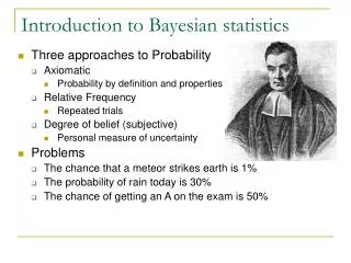
Probability vs. belief • What is a probability? • Frequentist point of view • Probabilities are what frequency counts (coin, die) and histograms (height of people) • Such definitions are somewhat circular because of the dependency on the Central Limit Theorem • Measure theory point of view • Probabilities satisfy Kolmogorov’s s-algebra axioms • Rigorous definition fits well within measure and integration theory • But definition is ad hoc to fit within this framework
Bayesian point of view • Probabilities are models of the uncertainty regarding propositions within a given domain • Induction vs. deduction • Deduction • IF ( A B AND A = TRUE )THEN B = TRUE • Induction • IF ( A B AND B = TRUE )THAN A becomes more plausible • Probabilities satisfy Bayes’ rule
The Cox-Jaynes axioms • The Cox-Jaynes axioms allow the buildup of a large probabilistic framework with minimal assumptions • Firstly, some concepts • A is a proposition • A TRUE or FALSE • D is a domain • Information available about the current situation • BELIEF: P(A=TRUE |D) • Belief that we have regarding the proposition given the domain knowledge
Secondly, some assumptions • Suppose we can compare beliefs • P(A|D) > P(B|D) Ais more plausible than B given D and suppose the comparison is transitive • We have an ordering relation, so P is a number
Suppose there exists a fixed relation between the belief in a proposition and the belief in the negation of this proposition • Suppose there exists a fixed relation between on the one hand the belief in the union of two propositions and on the other hand the belief in the first proposition and the belief in the second proposition given the first one
Bayes’ rule • THEN it can be shown (after rescaling of the beliefs) that • Bayes’ rule • If we accept the Cox-Jaynes axions, we can always apply Bayes’ rule, independently of the specific definition of the probabilities
Bayes’ rule • Bayes’ rule will be our main tool for building probabilistic models and to estimate them • Bayes’ rule holds not only for statements (TRUE/FALSE) but for any random variables (discrete or continuous) • Bayes’ rule holds for specific realizations of the random variables as well as for the whole distribution
Importance of the domain D • The domain D is a flexible concept that encapsulates the background information that is relevant for the problem • It is important to set up the problem within the right domain • Example • Diagnosis of Tay-Sachs’ disease • Rare disease that appears more frequently for Ashkenazi Jews • With the same symptoms, the probability of the disease will be smaller if we are in a hospital in Brussels that if we are in Mount Sinai Hospital in New York • If we try to build a model with all the patients in the world, this model will not be more efficient
Probabilistic models • We have a domain D • We have observations D • We have a model M with parameters q • Example 1 • Domain D: the genome of a given organism • Data D: a DNA sequence S = ’ACCTGATCACCCT’ • Model M: the sequences are generated by a discrete distribution over the alphabet {A,C,G,T} • Parameters q:
Example 2 • Domain D: all European people • Data D: the length of people from a given group • Model M: the length is normally distributed N(m,s) • Parameters q: the mean m and the standard deviation s
Generative models • It is often possible to set up a model of the likelihood of the data • For example, for the DNA sequence • More sophisticated models are possible • HMMs • Gibbs sampling for motif finding • Bayesian networks • We want to find the model that describes our observations
Maximum likelihood • Maximum likelihood (ML) • Consistent: if the observation were generated by the model M with parameters q*, then qML will converge to q* when the number of observations goes to infinity • Note that the data might not be generated by any instance of the model • If the data set is small, there might be a large difference between qML en q*
likelihood of the data posterior prior a priori knowledge plays no role inoptimization over q Maximum a posteriori probability • Maximum a posteriori probability (MAP) • Bayes’ rule • Thus
Posterior mean estimate • Posterior mean estimate
Length 150 175 200 150 5 Meanlength Standard deviationlength 175 10 200 15 Distributions over parameters • Let us look carefully to P(q|M) (or to P(q|D,M)) • P(q|M) is a probability distribution over the PARAMETERS • We have to handle both distributions over observations and over parameters at the same time • Example • Distribution of the length of people P(D|q,M) • Prior P(q|M)
1 3 2 Bayesian inference • If we want to update the probability of the parameters with new observations D • Choose a reasonable prior • Add the information from the data • Get the updated distributions of the parameters (We often work with logarithms)
100 Belgianmen Meanlength 150 175 200 100 Dutchmen Meanlength 150 175 200 Meanlength 150 175 200 Bayesian inference • Example
Marginalization • A major technique for working with probabilistic models is to introduce or remove a variable through marginalization wherever appropriate • If a variable Y can take only kmutually exclusive outcomes, we have • If the variables are continuous
Multinomial distribution • Discrete distribution • K independent outcomes with probabilities qi • Example • Die K=6 • DNA sequence K=4 • Amino acid sequence K=20 • For K=2 we have a Bernoulli variable (giving rise to a binomial distribution)
The multinomial distribution gives the number of times that the different outcomes were observed • The multinomial distribution is the natural distribution for the modeling of biological sequences
Dirichlet distribution • Distribution over the region of the parameter space where • The distribution has parameters • The Dirichlet distribution gives the probability of q • The distribution is like a ‘dice factory’
Dirichlet distribution • Z(a) is a normalization factor such that • G is de gamma function • Generalization of the factorial function to real numbers • The Dirichlet distribution is the natural prior for sequence analysis because this distribution is conjugate to the multinomial distribution, which means that if we have a Dirichlet prior and we update this prior with multinomial observations, the posterior will also have the form of a Dirichlet distribution • Computationally very attractive
GACGTG CTCGAG CGCGTG AACGTG CACGTG Count the number of instances in each column Estimation of frequency matrices • Estimation on the basis of counts • e.g., Position-Specific Scoring Matrix in PSI-BLAST • Example: matrix model of a local motif
If there are many aligned sites (N>>), we can estimate the frequencies as • This is the maximum likelihood estimate for q
Proof • We want to show that • This is equivalent to • Further
Pseudocounts • If we have a limited number of counts, the maximum likelihood estimate will not be reliable (e.g., for symbols not observed in the data) • In such a situation, we can combine the observations with prior knowledge • Suppose we use a Dirichlet prior q: • Let us compute the Bayesian update
Bayesian update =1 because both distributionsare normalized Computation of the posteriormean estimate Normalization integral Z(.)
Pseudocounts • Pseudocounts • The prior contributes to the estimation through pseudo-observations • If few observations are available, then the prior plays an important role • If many observations are available, then the pseudocounts play a negligible role
Dirichlet mixture • Sometimes the observations are generated by a heterogeneous process (e.g., hydrophobic vs. hydrophilic domains in proteins) • In such situations, we should use different priors in function of the context • But we do not necessarily know the context beforehand • A possibility is the use of a Dirichlet mixture • The frequency parameter q can be generated from m different sources S with different Dirichlet parameters ak
Dirichlet mixture • Posterior • Via Bayes’ rule
Dirichlet mixture • Posterior mean estimate • The different components of the Dirichlet mixture are first considered as separate pseudocounts • These components are then combined with a weight depending on the likelihood of the Dirichlet component
Summary • The Cox-Jaynes axioms • Bayes’ rule • Probabilistic models • Maximum likelihood • Maximum a posteriori • Bayesian inference • Multinomial and Dirichlet distributions • Estimation of frequency matrices • Pseudocounts • Dirichlet mixture