Download
1 / 8
181 likes | 561 Views
Bayesian statistics. Probabilities for everything. Different views on probability. Frequentistic : Probabilities are there to tell us about long-term frequencies. They are objective, solely properties of nature ( aleatoric ).

E N D
Bayesian statistics Probabilities for everything
Different views on probability Frequentistic: Probabilities are there to tell us about long-term frequencies. They are objective, solely properties of nature (aleatoric). Bayesian: Probabilities are there so that we can sum up our knowledge about things we are uncertain about. They are therefore found in the interplay between the subject of our study and ourselves. In Bayesian statistics, probabilities are subjective, but can obtain an air of weak objectivity (intersubjectivity) if most people can agree that these probabilities sum up their collective knowledge (example: dice).
Bayes formula Both latent variables and parameters are treated using probability theory. We treat everything with the same tool, conditional probabilities. In a sense, we only have observations and latent variables. Knowledge is updated using Bayes theorem: The probability density f() is called the prior and is meant to contain whatever information we have about before the data, in the form of a probability density. Restrictions on the possible values the parameters can take are placed here. More on this later. For discrete variables, replace the probability density, f, with probability and integrals with sums.
Bayes formula Bayes theorem: • This probability density, f(|D), is called the posterior distribution. It sums up everything we know about the parameters, , after dealing with the data, D. Estimates, parameter uncertainty, derived quantities, decision making and model testing all follows from this. • An estimate can be formed using the expectation, median or mode of the posterior distribution. • Parameter uncertainty can be described using credibility intervals. A 95% credibility interval (a,b) has the property Pr|D(a<<b)=95%. I .e. after the data, you have 95% probability of the parameter having a value inside this interval. • The distribution f(D) will turn out to be a (the?) problem.
Bayesian statistics – Pros / Cons • You *have* to supply a prior.That prior can be criticized. Making a prior that’s hard to criticize is hard. • Thinking about the meaning of a model parameter is extra work. • For some, frequentist probabilities make more sense than Bayesian ones. • Some think distinguishing between parameters and latent variables is important. • Sometimes you’re only interested in estimates. • Bayesian statistics is subjective (though it can be made inter-subjective with hard work). • Restrictions and insights coded in the prior from the biology can help the inference. • Since you need to give a prior, you are actually forced to think about the meaning of your model. • For some, Bayesian probabilities make more sense than frequentist ones. • You don’t have to take a stance on whether an unknown quantity is fundamentally stochastic or not. • You get the parameter uncertainty “for free”. • It can give answers where the classical approach has none (such as the occupancy probability conditioned only on the data). • You are actually allowed to talk about the probability that a parameter is found in a given interval and the probability of a given zero-hypothesis. (This is often how confidence intervals and p-values are incorrectly interpreted). • Understanding the output of a Bayesian analysis is often easier than for frequentist outputs.
Bayesian statistics vs frequentist statistics – the practical issue When the model or analysis complexity is below a certain limit, frequentist methods will be easier while above that threshold, Bayesian analysis is easier. Frequentist Work/ effort Bayesian Complexity
Graphical modelling - occupancy All unknown quantities are now on equal footing. All dependencies are described by conditional probabilities, with marginal probabilities (priors) at the top nodes. Prior: f()=1, f(p)=1 (,p~U(0,1), i.e. uniform between 0 and 1). p Parameters (): 1 2 3 A Latent variables: ……… Pr(i=1|)= The area occupancies are independent given the occupancy rate. Pr(xi,j=1 | i=1,)=p. Pr(xi,j=0 | i=1,)=1-p, Pr(xi,j=1 | i=0,)=0. Pr(xi,j=0 | i=0,)=1 x1,n1 x1,1 x1,2 ……… x1,3 Data:
Hyper-parameters If your prior has a parametric form, the stuff you put as values in these forms are the hyper-parameters. For instance, the uniform distribution from zero to one is a special case of a uniform prior from a to b. a,b ap,bp Prior: ~U(a,b) and p ~U(ap,bp). Since p and are rates, we have set a=ap=0, b=bp=1. Hyper-parameters: p Parameters (): 1 2 3 A ……… Latent variables: The hyper-parameters are fixed. They are there to sum up our prior knowledge. If you start doing inference on them, they are parameters, not hyper-parameters. x1,n1 x1,1 x1,2 ……… x1,3 Data: