Download
1 / 4
50 likes | 266 Views
Z and Laplace Transforms. Z and Laplace Transforms. Transform difference/differential equations into algebraic equations that are easier to solve Are complex-valued functions of a complex frequency variable Laplace: s = + j 2 f Z : z = r e j

E N D
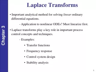
Z and Laplace Transforms • Transform difference/differential equations into algebraic equations that are easier to solve • Are complex-valued functions of a complex frequency variable Laplace: s = + j 2 f Z: z = rej • Transform kernels are complex exponentials Laplace: es t = e t +j 2 f t = e t ej 2 f t Z: zk = (rej)k= rkejk dampening factor oscillation term
f[k] H(z) y[k] Z Laplace H(s) Z and Laplace Transforms • No unique mapping from Z to Laplace domain or from Laplace to Z domain • Mapping one complex domain to another is not unique • One possible mapping is impulse invariance • Make impulse response of a discrete-time linear time-invariant (LTI) system be a sampled version of the continuous-time LTI system.
Im{z} 1 Re{z} Impulse Invariance Mapping • Impulse invariance mapping is z = e s T Im{s} 1 Re{s} -1 1 -1 s = -1 j z = 0.198 j 0.31 (T = 1 s) s = 1 j z = 1.469 j 2.287 (T = 1 s) lowpass, highpass bandpass, bandstop allpass, or notch filter?