Nspire CAS and Laplace Transforms

1. TIME 2014 Technology in MathematicsEducation July 1st - 5th2014, Krems, Austria Nspire CAS and Laplace Transforms Michel Beaudin, ÉTS, Montréal, Canada

2. Overview Introduction Two Specific Applications Mass-spring problem RLC circuit problem Piecewise and Impulse Inputs Using the convolution

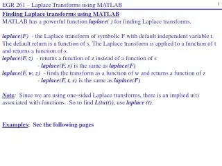
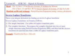
3. Introduction There is no built-in Laplace transform function in NspireCAS. But we can download an Nspire CAS library for using this stuff. For details about the Laplace transforms library “ETS_specfunc.tns”, see the document of Chantal Trottier: http://seg-apps.etsmtl.ca/nspire/documents/transf%20Laplace%20prog.pdf.

4. Introduction In this talk, we will use this Laplace transforms package to automate some engineering applications, such as mass-spring problem and RLC circuit. We will also use an animation: this helps students to get a better understanding of what is a “Dirac delta function”. Also, the convolution of the impulse response and the input willbeused to find the output in a RLC circuit withvarious input sources.

5. Introduction This is the pedagogical approach we have been using at ETS in the past 3 years with Nspire CAS CX handheld: using computer algebra to define functions. And encouraging students to define their own functions. These functions are saved into the library Kit_ETS_MB and can be downloaded from the webpage at: https://cours.etsmtl.ca/seg/MBEAUDIN/

6. Introduction The rest of this short Power Point file gives an overview of what will be done live, using Nspire CAS.

7. Two Specific Applications A damped mass-spring oscillator consists of an object of mass m attached to a spring fixed at one end. Applying Newton’s second law and Hooke’s law (let k denote the spring constant), adding some friction proportional to velocity (let b the factor) and an external force f(t), we will obtain a differential equation.

8. Two Specific Applications One can show that the position y(t) of the object satisfies the ODE Students are solving this problem using numeric values of the parameters m, b and k and various external forces f(t). The Laplace transform is applied to both sides of the ODE and, then, the inverse Laplace transform.

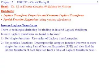
9. Two Specific Applications “Laplace transforms tables” are included in their textbook: students use the different properties to transform the ODE into an algebraic equation involving Y(s) (the Laplace transform of y(t)). The CAS handheld is used for partial fraction expansion. Term by term inverse transforms are found using the table.

10. Two Specific Applications The library ETS_specfunc is used to check their answers. This is how we have been proceeding at ETS since many years (TI-92 Plus, V200): for more details, see http://luciole.ca/gilles/conf/TIME-2010-Picard-Trottier-D014.pdf

11. Two Specific Applications Now we want to automate this process.Having gained confidence with Laplace transforms techniques, we solve by handwithout numeric values the ODE We find the following solution:

12. Two Specific Applications This is a function of 6 variables Why not define a “mass-spring” function? In French, “spring” is “ressort”: This is done in Nspire CAS using the “laplace” and “ilaplace” functions defined in the library ETS_specfunc(variables are necessary “t” and “s”).

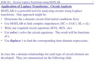
13. Two Specific Applications The same procedure can be applied to a series RLC circuit: we consider a voltage source E(t), a resistor R, an inductor L and a capacitor C. In this case, Kirchhoff’s voltage law (also Ohm’s law and Faraday’s law) are used to construct a model.

14. Two Specific Applications Textbooks give the details and the following ODE for the voltage across the capacitor is obtained: Here i(t) is the current at time t. The relation is given by

15. Two Specific Applications 1 The similitude with the former ODE can be exploited. So we can define a single function that solves this problem: Anotherfunction : of course,theorder of the variables could have been different.

16. Piecewise and Impulse Inputs Main reason why students are introduced to Laplace transforms techniques: to be able to consider piecewise external forces (or voltage sources). In order to do this, we first need to define the unit-step function u(t). Then we can define the rectangular pulse p(t).

17. Piecewise and Impulse Inputs Then, we can define the unit-impulse (or Dirac delta) function d(t) as follow: d(t) = 0 for t ≠ 0 d(t) is undefined for t = 0

18. Piecewise and Impulse Inputs Engineering students don’t need to be introduced to generalized functions. So instead of saying that the unit impulse is the derivative of the unit step function, we can use limiting arguments for a good understanding of this particular “function”. Here are the details.

19. Piecewise and Impulse Inputs Let abe a non negative fixed number. Let e > 0. Use the rectangular pulse function Note that this is a scaled indicator function of the interval a < t < a + e.

20. Piecewise and Impulse Inputs A good method to really understand what is the meaning of the Dirac delta function would be to use a limiting process. Example: we will consider We will solve this directly using the “ressort” function defined earlier.

21. Piecewise and Impulse Inputs But we will also solve the ODE Then, we will animate the solution, starting with e = 1 and getting closer to 0. This is, in fact, the main idea behind an impulse function.

22. Using the convolution Finally, consider the ODE Let h(t) be the inverse Laplace transform of the so called transfer function: Then the solution of the ODE is given by

23. Using the convolution A word about the integral This is called the convolution of the input x(t) with the impulse response h(t).This impulse response is entirely determined by the components of the system.

24. Using the convolution Fortunately, in the case of Laplace transforms, we don’t have to compute the integral in order to find the convolution of two signals x(t) and h(t). Instead, we use the “convolution property”:

25. Using the convolution Convolution of signals is already defined inETS_specfunc. We have decided to use a different name to make the distinction with the general convolution of signals. In Kit_ETS_MB, “convolap(x, h)” simplifies to the convolution of signals x(t) and h(t) in the Laplace transform sense, using the functions “Laplace” and “Ilaplace” of ETS_specfunc.

26. Using the convolution We will use this fact to find the output in a RLC circuit with various voltage sources. Linearity and time invariance will be illustrated (notion of a “LTI system”).

27. Using the convolution We will use this fact to find the output in a RLC circuit with various voltage sources. Linearity and time invariance will be illustrated (notion of a “LTI system”).

28. Using the convolution Now, let’s switch to Nspire CAS and show the examplesto conclude this talk.

29. Thank You!