Download
1 / 48
500 likes | 710 Views
MSc Remote Sensing 2006-7 Principles of Remote Sensing 5: resolution II angular/temporal. Dr. Hassan J. Eghbali. Recap. Previously introduced spatial and spectral resolution narrow v broad band tradeoffs.... signal to noise ratio This week temporal and angular resolution

E N D
MSc Remote Sensing 2006-7Principles of Remote Sensing 5: resolution II angular/temporal Dr. Hassan J. Eghbali
Recap • Previously introduced • spatial and spectral resolution • narrow v broad band tradeoffs.... • signal to noise ratio • This week • temporal and angular resolution • orbits and sensor swath • radiometric resolution Dr. Hassan J. Eghbali
Temporal • Single or multiple observations • How far apart are observations in time? • One-off, several or many? • Depends (as usual) on application • Is it dynamic? • If so, over what timescale? Useful link: http://www.earth.nasa.gov/science/index.html Dr. Hassan J. Eghbali
Temporal • Examples • Vegetation stress monitoring, weather, rainfall • hours to days • Terrestrial carbon, ocean surface temperature • days to months to years • Glacier dynamics, ice sheet mass balance, erosion/tectonic processes • Months to decades Useful link: http://www.earth.nasa.gov/science/index.html Dr. Hassan J. Eghbali
What determines temporal sampling? • Sensor orbit • geostationary orbit - over same spot • BUT distance means entire hemisphere is viewed e.g. METEOSAT • polar orbit can use Earth rotation to view entire surface • Sensor swath • Wide swath allows more rapid revisit • typical of moderate res. instruments for regional/global applications • Narrow swath == longer revisit times • typical of higher resolution for regional to local applications Dr. Hassan J. Eghbali
Orbits and swaths • Orbital characteristics • orbital mechanics developed by Johannes Kepler (1571-1630), German mathematician • Explained observations of Danish nobleman Tyco Brahe (1546-1601) • Kepler favoured elliptical orbits (from Copernicus’ solar-centric system) • Properties of ellipse? Dr. Hassan J. Eghbali
r1 r2 2b minor axis f2 f1 C • ecircle = 0 • As e 1, c a and ellipse becomes flatter Increasing eccentricity 2c 2a major axis Ellipse • Flattened circle • 2 foci and 2 axes: major and minor • Distance r1+r2 = constant = 2a (major axis) • “Flatness” of ellipse defined by eccentricity, e = 1-b2/a2 = c/a • i.e. e is position of the focus as a fraction of the semimajor axis, a From http://mathworld.wolfram.com/Ellipse.html Dr. Hassan J. Eghbali
Kepler’s laws • Kepler’s Laws • deduced from Brahe’s data after his death • see nice Java applet http://www-groups.dcs.st-and.ac.uk/~history/Java/Ellipse.html • Kepler’s 1st law: • Orbits of planets are elliptical, with sun at one focus From:http://csep10.phys.utk.edu/astr161/lect/history/kepler.html Dr. Hassan J. Eghbali
Kepler’s laws • Kepler’s 2nd law • line joining planet to sun sweeps out equal areas in equal times From:http://csep10.phys.utk.edu/astr161/lect/history/kepler.html Dr. Hassan J. Eghbali
Kepler’s laws • Kepler’s 3rd law • “ratio of the squares of the revolutionary periods for two planets (P1, P2) is equal to the ratio of the cubes of their semimajor axes (R1, R2)” • P12/P22 = R13/R23 • i.e. orbital period increases dramatically with R • Convenient unit of distance is average separation of Earth from Sun = 1 astronomical unit (A.U.) • 1A.U. = 149,597,870.691 km • in Keplerian form, P(years)2 R(A.U.)3 • or P(years) R(A.U.)3/2 • or R(A.U.) P(years)2/3 Dr. Hassan J. Eghbali
Orbits: examples • Orbital period for a given instrument and height? • Gravitational force Fg = GMEms/RsE2 • G is universal gravitational constant (6.67x10⁻¹¹ Nm2kg2); ME is Earth mass (5.983x1024kg); ms is satellite mass (?) and RsE is distance from Earth centre to satellite i.e. 6.38x10⁶ + h where h is satellite altitude • Centripetal (not centrifugal!) force Fc = msvs2/RsE • where vs is linear speed of satellite (=sRsE where is the satellite angular velocity, rad s-1) • for stable (constant radius) orbit Fc = Fg • GMEms/RsE2 = msvs2/RsE = ms s2RsE2 /RsE • so s2 = GME /RsE3 Dr. Hassan J. Eghbali
Orbits: examples • Orbital period T of satellite (in s) = 2/ • (remember 2 = one full rotation, 360°, in radians) • and RsE = RE + h where RE = 6.38x10⁶ m • So now T = 2[(RE+h)3/GME]1/2 • Example: polar orbiter period, if h = 705x103m • T = 2[(6.38x10⁶ +705x103)3 / (6.67x10-11*5.983x1024)]1/2 • T = 5930.6s = 98.8mins • Example: altitude for geostationary orbit? T = ?? • Rearranging: h = [(GME /42)T2 ]1/3 - RE • So h = [(6.67x10-11*5.983x1024/42)(24*60*60)2 ]1/3 - 6.38x10⁶ • h = 42.2x10⁶ - 6.38x106 = 35.8km Dr. Hassan J. Eghbali
l r Orbits: aside • Convenience of using radians • By definition, angle subtended by an arc (in radians) = length of arc/radius of circle i.e. = l/r • i.e. length of an arc l = r • So if we have unit circle (r=1), l = circumference = 2r = 2 • So, 360° = 2 radians Dr. Hassan J. Eghbali
Orbital pros and cons • Geostationary? • Circular orbit in the equatorial plane, altitude ~36,000km • Orbital period? • Advantages • See whole Earth disk at once due to large distance • See same spot on the surface all the time i.e. high temporal coverage • Big advantage for weather monitoring satellites - knowing atmos. dynamics critical to short-term forecasting and numerical weather prediction (NWP) • GOES (Geostationary Orbiting Environmental Satellites), operated by NOAA (US National Oceanic and Atmospheric Administration) • http://www.noaa.gov/ and http://www.goes.noaa.gov/ Dr. Hassan J. Eghbali
GOES-E 75° W GOES-W 135° W METEOSAT 0° W IODC 63° E GMS 140° E Geostationary • Meteorological satellites - combination of GOES-E, GOES-W, METEOSAT (Eumetsat), GMS (NASDA), IODC (old Meteosat 5) • GOES 1st gen. (GOES-1 - ‘75 GOES-7 ‘95); 2nd gen. (GOES-8++ ‘94) From http://www.sat.dundee.ac.uk/pdusfaq.html Dr. Hassan J. Eghbali
Geostationary • METEOSAT - whole earth disk every 15 mins From http://www.goes.noaa.gov/f_meteo.html Dr. Hassan J. Eghbali
Geostationary orbits • Disadvantages • typically low spatial resolution due to high altitude • e.g. METEOSAT 2nd Generation (MSG) 1x1km visible, 3x3km IR (used to be 3x3 and 6x6 respectively) • MSG has SEVIRI and GERB instruments • http://www.meteo.pt/landsaf/eumetsat_sat_char.html • Cannot see poles very well (orbit over equator) • spatial resolution at 60-70° N several times lower • not much good beyond 60-70° • NB Geosynchronous orbit same period as Earth, but not equatorial From http://www.esa.int/SPECIALS/MSG/index.html Dr. Hassan J. Eghbali
Polar & near polar orbits • Advantages • full polar orbit inclined 90 to equator • typically few degrees off so poles not covered • orbital period typically 90 - 105mins • near circular orbit between 300km (low Earth orbit) and 1000km • typically higher spatial resolution than geostationary • rotation of Earth under satellite gives (potential) total coverage • ground track repeat typically 14-16 days From http://collections.ic.gc.ca/satellites/english/anatomy/orbit/ Dr. Hassan J. Eghbali
(near) Polar orbits: NASA Terra From http://visibleearth.nasa.gov/cgi-bin/viewrecord?134 Dr. Hassan J. Eghbali
Near-polar orbits: Landsat • inclination 98.2, T = 98.8mins • http://www.cscrs.itu.edu.tr/page.en.php?id=51 • http://landsat.gsfc.nasa.gov/project/Comparison.html From http://www.iitap.iastate.edu/gccourse/satellite/satellite_lecture_new.html & http://eosims.cr.usgs.gov:5725/DATASET_DOCS/landsat7_dataset.html Dr. Hassan J. Eghbali
(near) Polar orbits • Disadvantages • need to launch to precise altitude and orbital inclination • orbital decay • at LEOs (Low Earth Orbits) < 1000km, drag from atmosphere • causes orbit to become more eccentric • Drag increases with increasing solar activity (sun spots) - during solar maximum (~11yr cycle) drag height increased by 100km! • Build your own orbit: http://lectureonline.cl.msu.edu/~mmp/kap7/orbiter/orbit.htm From http://collections.ic.gc.ca/satellites/english/anatomy/orbit/ Dr. Hassan J. Eghbali
Types of near-polar orbit • Sun-synchronous • Passes over same point on surface at approx. same local solar time each day (e.g. Landsat) • Characterised by equatorial crossing time (Landsat ~ 10am) • Gives standard time for observation • AND gives approx. same sun angle at each observation • good for consistent illumination of observations over time series (i.e. Observed change less likely to be due to illumination variations) • BAD if you need variation of illumination (angular reflectance behaviour) • Special case is dawn-to-dusk • e.g. Radarsat 98.6° inclination • trails the Earth’s shadow (day/night border) • allows solar panels to be kept in sunlight all the time) Dr. Hassan J. Eghbali
Near-ish: Equatorial orbit • Inclination much lower • orbits close to equatorial • useful for making observations solely over tropical regions • Example • TRMM - Tropical Rainfall Measuring Mission • Orbital inclination 35.5°, periapsis (near point: 366km), apoapsis (far point: 3881km) • crosses equator several times daily • Flyby of Hurrican Frances (24/8/04) • iso-surface From http://trmm.gsfc.nasa.gov/ Dr. Hassan J. Eghbali
Orbital location? • TLEs (two line elements) • http://www.satobs.org/element.html e.g. PROBA 1 1 26958U 01049B 04225.33423432 .00000718 00000-0 77853-4 0 2275 2 26958 97.8103 302.9333 0084512 102.5081 258.5604 14.88754129152399 • DORIS, GPS, Galileo etc. • DORIS: Doppler Orbitography and Radiopositioning Integrated by Satellite • Tracking system providing range-rate measurements of signals from a dense network of ground-based beacons (~cm accuracy) • GPS: Global Positioning System • http://www.vectorsite.net/ttgps.html • http://www.edu-observatory.org/gps/tracking.html Dr. Hassan J. Eghbali
direction of travel satellite ground swath one sample two samples three samples Instrument swath • Swath describes ground area imaged by instrument during overpass Dr. Hassan J. Eghbali
MODIS on-board Terra From http://visibleearth.nasa.gov/cgi-bin/viewrecord?130 Dr. Hassan J. Eghbali
Terra instrument swaths compared From http://visibleearth.nasa.gov/Sensors/Terra/ Dr. Hassan J. Eghbali
Broad swath • MODIS, POLDER, AVHRR etc. • swaths typically several 1000s of km • lower spatial resolution • Wide area coverage • Large overlap obtains many more view and illumination angles (much better termporal & angular (BRDF) sampling) • Rapid repeat time Dr. Hassan J. Eghbali
MODIS: building global picture • Note across-track “whiskbroom” type scanning mechanism • swath width of 2330km (250-1000m resolution) • Hence, 1-2 day repeat cycle From http://visibleearth.nasa.gov/Sensors/Terra/ Dr. Hassan J. Eghbali
AVHRR: global coverage • 2400km swath, 1.1km pixels at nadir, but > 5km at edge of swath • Repeats 1-2 times per day From http://edc.usgs.gov/guides/avhrr.html Dr. Hassan J. Eghbali
POLDER (RIP!) • Polarisation and Directionality of Earth’s Reflectance • FOV ±43° along track, ±51° across track, 9 cameras, 2400km swath, 7x6km resn. at nadir • POLDER I 8 months, POLDER II 7 months.... Each set of points corresponds to given viewing zenith and azimuthal angles for near-simultaneous measurements over a region defined by lat 0°±0.5° and long of 0°±0.5° (Nov 1996) Each day, region is sampled from different viewing directions so hemisphere is sampled heavily by compositing measurements over time From Loeb et al. (2000) Top-of-Atmosphere Albedo Estimation from Angular Distribution Models Using Scene Identification from Satellite Cloud Property Retrievals, Journal of Climate, 1269-1285. From http://www-loa.univ-lille1.fr/~riedi/BROWSES/200304/16/index.html Dr. Hassan J. Eghbali
Narrow swath • Landsat TM/MSS/ETM+, IKONOS, QuickBird etc. • swaths typically few 10s to 100skm • higher spatial resolution • local to regional coverage NOT global • far less overlap (particularly at lower latitudes) • May have to wait weeks/months for revisit Dr. Hassan J. Eghbali
Landsat: local view • 185km swath width, hence 16-day repeat cycle (and spatial res. 25m) • Contiguous swaths overlap (sidelap) by 7.3% at the equator • Much greater overlap at higher latitudes (80% at 84°) From http://visibleearth.nasa.gov/Sensors/Terra/ Dr. Hassan J. Eghbali
QuickBird: 16.5km swath at nadir, 61cm! panchromatic, 2.44m multispectral • http://www.digitalglobe.com • IKONOS: 11km swath at nadir, 1m panchromatic, 4m multispectral • http://www.spaceimaging.com/ IKONOS & QuickBird: very local view! Dr. Hassan J. Eghbali
Variable repeat patterns • ERS 1 & 2 • ATSR instruments, RADAR altimeter, Imaging SAR (synthetic aperture RADAR) etc. • ERS 1: various mission phases: repeat times of 3 (ice), 35 and 168 (geodyssey) days • ERS 2: 35 days From http://earth.esa.int/rootcollection/eeo/ERS1.1.7.html Dr. Hassan J. Eghbali
So.....angular resolution • Wide swath instruments have large overlap • e.g. MODIS 2330km (55), so up to 4 views per day at different angles! • AVHRR, SPOT-VGT, POLDER I and II, etc. • Why do we want good angular sampling? • Remember BRDF? • http://stress.swan.ac.uk/~mbarnsle/pdf/barnsley_et_al_1997.pdf • Information in angular signal! • More samples of viewing/illum. hemisphere gives more info. Dr. Hassan J. Eghbali
relative azimuth (view - solar) view zenith Cross solar principal plane Solar principal plane Angular sampling: broad swath • MODIS and SPOT-VGT: polar plots • http://www.soton.ac.uk/~epfs/methods/polarplot.shtml • Reasonable sampling BUT mostly across principal plane (less angular info.) • Is this “good” sampling of BRDF Dr. Hassan J. Eghbali
Angular sampling: broad swath • POLDER I ! • Broad swath (2200km) AND large 2D CCD array gave huge number of samples • 43 IFOV along-track and 51 IFOV across-track Dr. Hassan J. Eghbali
BUT....... • Is wide swath angular sampling REALLY multi-angular? • Different samples on different days e.g. MODIS BRDF product is composite over 16 days • minimise impact of clouds, maximise number of samples • “True” multi-angular viewing requires samples at same time • need to use several looks e.g. ATSR, MISR (& POLDER) Dr. Hassan J. Eghbali
Angular sampling: narrow swath • ATSR-2 and MISR polar plots • Better sampling in principal plane (more angular info.) • MISR has 9 cameras Dr. Hassan J. Eghbali
Angular sampling: combinations? • MODIS AND MISR: better sampling than either individually • Combine observations to sample BRDF more effectively Dr. Hassan J. Eghbali
So, angular resolution • Function of swath and IFOV • e.g. MODIS at nadir ~1km pixel • remember l = r so angle (in rads) = r/l where r this time is 705km and l ~ 1km so angular res ~ 1.42x10⁻⁶ rads at nadir • at edge of swath ~5km pixel so angular res ~ 7x10⁻⁶ rads • Sampling more important/meaningful than resolution in angular sense... Dr. Hassan J. Eghbali
Radiometric resolution • Had spatial, spectral, temporal, angular..... • Precision with which an instrument records EMR • i.e. Sensitivity of detector to amount of incoming radiation • More sensitivity == higher radiometric resolution • determines smallest slice of EM spectrum we can assign DN to • BUT higher radiometric resolution means more data • As is the case for spatial, temporal, angular etc. • Typically, radiometric resolution refers to digital detectors • i.e. Number of bits per pixel used to encode signal Dr. Hassan J. Eghbali
Radiometric resolution • Analogue • continuous measurement levels • film cameras • radiometric sensitivity of film emulsion • Digital • discrete measurement levels • solid state detectors (e.g. semiconductor CCDs) Dr. Hassan J. Eghbali
1 to 6 bits (left to right) • black/white (21) up to 64 graylevels (26) (DN values) • human eye cannot distinguish more than 20-30 DN levels in grayscale i.e. ‘radiometric resolution’ of human eye 4-5 bits Radiometric resolution • Bits per pixel • 1 bit (0,1); 2bits (0, 1, 2, 3); 3 bits (0, 1, 2, 3, 4, 5, 6, 7) etc. • 8 bits in a byte so 1 byte can record 28 (256) different DNs (0-255) From http://ceos.cnes.fr:8100/cdrom/ceos1/irsd/pages/dre4.htm Dr. Hassan J. Eghbali
Radiometric resolution: examples • Landsat: MSS 7bits, TM 8bits • AVHRR: 10-bit (210 = 1024 DN levels) • TIR channel scaled (calibrated) so that DN 0 = -273°C and DN 1023 ~50°C • MODIS: 12-bit (212 = 4096 DN levels) • BUT precision is NOT accuracy • can be very precise AND very inaccurate • so more bits doesn’t mean more accuracy • Radiometric accuracy designed with application and data size in mind • more bits == more data to store/transmit/process Dr. Hassan J. Eghbali
Summary: angular, temporal resolution • Coverage (hence angular &/or temporal sampling) due to combination of orbit and swath • Mostly swath - many orbits nearly same • MODIS and Landsat have identical orbital characteristics: inclination 98.2°, h=705km, T = 99mins BUT swaths of 2400km and 185km hence repeat of 1-2 days and 16 days respectively • Most EO satellites typically near-polar orbits with repeat tracks every 16 or so days • BUT wide swath instrument can view same spot much more frequently than narrow • Tradeoffs again, as a function of objectives Dr. Hassan J. Eghbali
Summary: radiometric resolution • Number of bits per pixel • more bits, more precision (not accuracy) • but more data to store, transmit, process • most EO data typically 8-12 bits (in raw form) • Tradeoffs again, as a function of objectives Dr. Hassan J. Eghbali