Download
1 / 29
380 likes | 727 Views
Conjugate Gradient. 0. History. Why iterate? Direct algorithms require O(n³) work. 1950: n=20 1965: n=200 1980: n=2000 1995: n=20000. dimensional increase: 10 3 computer hardware: 10 9. 0. History. If matrix problems could be solved in O(n²) time , matrices could be 30 bigger.

E N D
0. History • Why iterate? • Direct algorithms require O(n³) work. • 1950: n=20 • 1965: n=200 • 1980: n=2000 • 1995: n=20000 dimensional increase: 103 computer hardware: 109
0. History • If matrix problems could be solved in O(n²) time, matrices could be 30 bigger. • There are direct algorithms that run in about O(n2.4) time, but their constant factors are to big for practicle use. • For certain matrices, iterative methods have the potential to reduce computation time to O(m²).
1. Introduction • CG is the most popular method for solving large systems of linear equationsAx = b. • CG is an iterative method, suited for use with sparse matrices with certain properties. • In practise, we generally don’t find dense matrices of a huge dimension, since the huge matrices often arise from discretisation of differential of integral equations.
2. Notation • Matrix: A, with components Aij • Vector, n x 1 matrix: x, with components xi • Linear equation: Ax=bwith components ΣAij xj = bi
2. Notation • Transponation of a matirx: (AT)ij = Aji • Inner product of two vectors: xTy = Σ xiyi • If xTy = 0, then x and y are orthogonal
3. Properties of A • A has to be an n x n matrix. • A has to be positive definite, xTAx > 0 • A has to be symmetric, AT = A
4. Quadratic Forms • A QF is a scalar quadratic function of a vector: • Example:
4. Quadratic Forms • Gradient: Points to the greatest increase of f(x)
4. Quadratic Forms positive definite xT A x > 0 negative definite xT A x < 0 positive indefinite xT A x≥ 0 indefinite
5. Steepest Descent • Start at an arbitrary point and slide down to the bottom of the paraboloid. • Steps x(1), x(2), … in the direction –f´(xi) • Error e(i) = x(i) – x • Residual r(i) = b – Ax(i) r(i) = - Ae(i) r(i) = - f`(x(i))
5. Steepest Descent • x(i+1) = x(i) + α r(i) , but how big is α? • f`(x(i+1)) orthogonal to r(i) search line α r(i)
5. Steepest Descent The algorithm above requires two matrix multiplications per iteration. One can be eliminated by multiplying the last equation by –A.
5. Steepest Descent This sequence is generated without any feedback of x(i). Therefore, floatingpoint roundoff errors may accumulate and the sequence could converge at some point near x. This effect can be avoided by periodically recomputing the correct residual using x(i).
6. Eigenvectors • v is an eigenvector of A, if a scalar λ so that A v = λ v • λ is then called an eigenvalue. • A symmetric n x n matrix always has n independent eigenvectors which are orthogonal. • A positive definite matrix has positive eigenvalues.
7. Convergence of SD • Convergence of SD requires the error e(i) to vanish. To measure e(i), we use the A- norm: • Some math now yields
7. Convergence of SD Spectral condition number . An upper bound for ω is found by setting . We therefore have instant convergence if all the eigenvalues of A are the same.
7. Convergence of SD large κ small μ large κ large μ small κ large μ small κ small μ
8. Conjugate Directions • Steepest Descent often takes steps in the same direction as earlier steps. • The solution is to take a set of A-orthogonal search directions d(0), d(1), … , d(n-1) and take exactly one step of the right length in each direction.
8. Conjugate Directions A-orthogonal orthogonal
8. Conjugate Directions • Demanding dT(i) to be A-orthogonal on the next error e(i+1), we get . • Generating search directions by Gram-Schmidt Conjugation. Problem: O(n³)
8. Conjugate Directions • CD chooses , so thatis minimized. • The error term is therefore A-orthogonal to all the old search directions.
9. Conjugate Gradient • The residual is orthogonal to the previous search directions. • Krylov subspace
9. Conjugate Gradient • Gram-Schmidt conjugation becomes easy, because r(i+1) is already A-orthogonal to all the previous search directions except d(i). r(i+1) is A-orthogonal to Di
11. Preconditioning • Improving the condition number of the matrix before the calculation. Example: • Attempt to strech the quadratic form to make it more spherical. • Many more sophisticated preconditioners have been developed and are nearly always used.
12. Outlook • CG can also be used to solve • To solve non-linear Problems with CG, one has to make changes in the algorithm. There are several possibilities, and the best choice is still under research. .
12. Outlook In non-linear problems, there may be several local minima to which CG might converge. It is therefore hard to determine the right step size.
12. Outlook • There are other algorithms in numerical linear algebra closely related to CG. • They all use Krylov subspaces.