Gradient

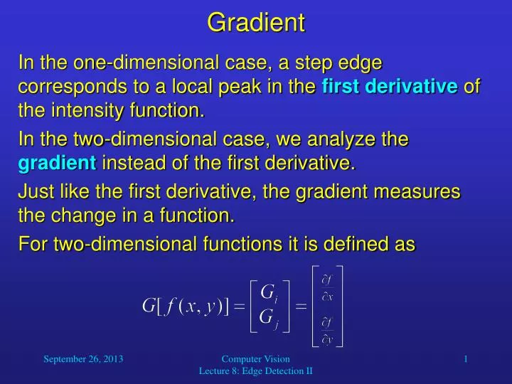
1. Gradient • In the one-dimensional case, a step edge corresponds to a local peak in the first derivative of the intensity function. • In the two-dimensional case, we analyze the gradient instead of the first derivative. • Just like the first derivative, the gradient measures the change in a function. • For two-dimensional functions it is defined as Computer Vision Lecture 8: Edge Detection II

2. Gradient • Gradients of two-dimensional functions: The two-dimensional function in the left diagram is represented by contour lines in the right diagram, where arrows indicate the gradient of the function at different locations. Obviously, the gradient is always pointing in the direction of the steepest increase of the function. Computer Vision Lecture 8: Edge Detection II

3. 1 Gi= Gj= 1 -1 -1 Gradient • In order to compute Gx and Gy in an image F at position [i, j], we need to consider the discrete case and get: • Gi = F[i+1, j] – F[i, j] • Gj = F[i, j+1] – F[i, j] • This can be done with convolution filters: To be precise in the assignment of gradients to pixels and to reduce noise, we usually apply 33 filters instead (next slide). Computer Vision Lecture 8: Edge Detection II

4. 1 0 -1 1 2 1 2 0 -2 0 0 0 1 0 -1 -1 -2 -1 Sj Si Sobel Filters • Sobel filters are the most common variant of edge detection filters. • Two small convolution filters are used successively: Computer Vision Lecture 8: Edge Detection II

5. Sobel Filters • Sobel filters yield two interesting pieces of information: • The magnitude of the gradient (local change in brightness): • The angle of the gradient (tells us about the orientation of an edge): Computer Vision Lecture 8: Edge Detection II

6. Sobel Filters Calculating the magnitude of the brightness gradient with a Sobel filter. Left: original image; right: filtered image. Computer Vision Lecture 8: Edge Detection II

7. Laplacian Filters • Let us take a look at the one-dimensional case: • A change in brightness: • Its first derivative: • Its second derivative: Computer Vision Lecture 8: Edge Detection II

8. Laplacian Filters • Idea: • Smooth the image, • compute the second derivative of the (2D) image, • Find the pixels where the brightness function “crosses” 0 and mark them. • We can actually devise convolution filters that carry out the smoothing and the computation of the second derivative. Computer Vision Lecture 8: Edge Detection II

9. Laplacian Filters Computer Vision Lecture 8: Edge Detection II

10. Laplacian Filters • Since we want the computation centered at [i,j]: Obviously, each function can be computed using a 1, -2, 1 convolution filter in horizontal or vertical direction. Since 2 is defined as the sum of these two functions, we can use a single 33 (or larger) convolution filter for its computation (next slide). Computer Vision Lecture 8: Edge Detection II

11. Laplacian Filters • Continuous variant: Discrete variants(applied after smoothing): Computer Vision Lecture 8: Edge Detection II

12. Laplacian Filters • Let us apply a Laplacian filter to the same image: Computer Vision Lecture 8: Edge Detection II

13. 55 Laplacian 77 Laplacian zero detection zero detection zero detection Laplacian Filters • 33 Laplacian Computer Vision Lecture 8: Edge Detection II

14. Gaussian Edge Detection • As you know, one of the problems in edge detection is the noise in the input image. • Noise creates lots of local intensity gradients that can trigger unwanted responses by edge detection filters. • We can reduce noise through (Gaussian) smoothing, but there is a trade-off: • Stronger smoothing will remove more of the noise, but will also add uncertainty to the location of edges. • For example, if two parallel edges are close to each other and we use a strong (i.e., large) Gaussian filter, these edges may be merged into one. Computer Vision Lecture 8: Edge Detection II

15. Canny Edge Detector • The Canny edge detector is a good approximation of the optimal operator, i.e., the one that maximizes the product of signal-to-noise ratio and localization. • Basically, the Canny edge detector is the first derivative of a Gaussian function. • Let I[i, j] be our input image. • We apply our usual Gaussian filter with standard deviation  to this image to create a smoothed image S[i, j]: • S[i, j] = G[i, j; ] * I[i, j] Computer Vision Lecture 8: Edge Detection II

16. Canny Edge Detector • In the next step, we take the smoothed array S[i, j] and compute its gradient. • We apply 22 filters to approximate the vertical derivative P[i, j] and the horizontal derivative Q[i, j]: • P[i, j]  (S[i+1, j] – S[i, j] + S[i+1, j+1] – S[i, j+1])/2 • Q[i, j]  (S[i, j+1] – S[i, j] + S[i+1, j+1] – S[i+1, j])/2 • As you see, we average over the 22 square so that the point for which we compute the gradient is the same for the horizontal and vertical components(the center of the 22 square). Computer Vision Lecture 8: Edge Detection II

17. 0.5 0.5 0.5 -0.5 P: Q: -0.5 -0.5 0.5 -0.5 Canny Edge Detector • P and Q can be computed using 22 convolution filters: We use the upper left element as the reference point of the filter. That means when we place the filter on the image, the location of the upper left element indicates where to enter the resulting value into the new image. Computer Vision Lecture 8: Edge Detection II

18. Canny Edge Detector • Once we have computed P[i, j] and Q[i, j], we can also compute the magnitude and orientation of the gradient vector at position [i, j]: This is exactly the information that we want – it tells us where edges are, how significant they are, and what their orientation is. However, this information is still very noisy. Computer Vision Lecture 8: Edge Detection II

19. Canny Edge Detector • The first problem is that edges in images are not usually indicated by perfect step edges in the brightness function. • Brightness transitions usually have a certain slope that extends across many pixels. • As a consequence, edges typically lead to wide lines of high gradient magnitude. • However, we would like to find thin lines that most precisely describe the boundary between two objects. • This can be achieved with the nonmaxima suppression technique. Computer Vision Lecture 8: Edge Detection II

20. 180 0 0 225 135 1 3 1 3 2 2 270 90 2 2 3 1 3 315 1 45 0 0 0 Canny Edge Detector • We first assign a sector [i, j] to each pixel according to its associated gradient orientation [i, j]. • There are four sectors with numbers 0, …, 3: Computer Vision Lecture 8: Edge Detection II

21. Canny Edge Detector • Then we iterate through the array M[i, j] and compare each element to two of its 8-neighbors. • Which two neighbors we choose depends on the value of [i, j]. • In the following diagram, the numbers in the neighboring squares of [i, j] indicate the value of [i, j] for which these neighbors are chosen: Computer Vision Lecture 8: Edge Detection II

22. Canny Edge Detector • If the value of M[i, j] is less than either of the M-values in these two neighboring positions, set E[i, j] = 0. • Otherwise, set E[i, j] = M[i, j]. • The resulting array E[i, j] is of the same size as M[i, j] and contains values greater than zero only at local maxima of gradient magnitude (measured in local gradient direction). • Notice that an edge in an image always induces an intensity gradient that is perpendicular to the orientation of the edge. • Thus, this nonmaxima suppression technique thins the detected edges to a width of one pixel. Computer Vision Lecture 8: Edge Detection II