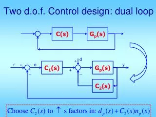
Two d.o.f. Control design: dual loop
550 likes | 680 Views
Two d.o.f. Control design: dual loop. C(s). G p (s). d. +. r. +. e. C 1 (s). G p (s). y. +. _. _. C 2 (s). Example from last time: Two different implementations:. sy. y. PI*PD +0.1s. _. _. -0.1. Standard. PD +0.1s. y. PI. _. _. -0.1. Alternative (more overshoot).

Two d.o.f. Control design: dual loop
E N D
Presentation Transcript
Two d.o.f. Control design: dual loop C(s) Gp(s) d + r + e C1(s) Gp(s) y + _ _ C2(s)
Example from last time: Two different implementations: sy y PI*PD +0.1s _ _ -0.1 Standard PD +0.1s y PI _ _ -0.1 Alternative (more overshoot)
Two d.o.f. Control design: FF+FB C(s) Gp(s) Cf(s) d + + r + e C(s) Gp(s) y + + _
Example: Cf(s) d + + r + e C(s) y + + _ Suppose C(s) is a lead-lag controller. Without Cf, what is the system type w.r.t. r? What is the system type w.r.t. d? Can Cf affect the type w.r.t. d? Can Cf affect the type w.r.t. r?
Example: Cf(s) d + + r + e C(s) y + + _ Suppose C(s) is a lead-lag controller. Q: Find a Cf to achieve 0 ess tracking for ramp input.
Cf(s) d + + r + e C(s) y + + _
Design specs: use PID to achieve Ess to ramp input = 0 As fast as possible Overshoot <= 25% Plant is type 1, so need PI after PD. 25% Mp PM >= 45, but with PI, need PMd 55 PD can contribute a maximum of about 75 So, select max wgc at phase=-200
s=tf('s'); Gp=1/s/(s+1)/(s+5); figure(2); margin(Gp); grid; V=axis; Mp=25; PMd = 70 - Mp + 10; %+10 for PI later DPM=75; PM=PMd-DPM; hold on; plot([V(1) V(2)],[PM PM]-180,'r:'); [x, y]=ginput(1); wgcd=x; z_PD = wgcd/tan(DPM*pi/180); %PD control K = 1/abs(evalfr((s+z_PD)*Gp,j*wgcd)); C=K*(s+z_PD); margin(C*Gp); grid; %Bode with PD z_PI = wgcd/10; C=C*(s+z_PI)/s; %multiply PI and PD margin(C*Gp); grid; hold off; %Bode with PID t=linspace(0, 15/wgcd, 301); figure(3); step(C*Gp/(1+C*Gp),t); grid;
Figure 8-8 Unit-step response curve of PID-controlled system designed by use of the Ziegler–Nichols tuning rule (second method).
Figure 8-10 Unit-step response of the system shown in Figure 8–6 with PID controller after numerical tuning of PID parameters.
Observations: Can shift red bump toward high freq a bit to increase speed But at higher freq, phase is lower, so PD needs to contribute more DPM PM=48 can be reduced by about 3
s=tf('s'); Gp=1/s/(s+1)/(s+5); figure(2); margin(Gp); grid; V=axis; Mp=25; PMd = 70 - Mp+ 7; %+7 for PI later DPM=85; PM=PMd-DPM; hold on; plot([V(1) V(2)],[PM PM]-180,'r:'); [x, y]=ginput(1); wgcd=x; z_PD = wgcd/tan(DPM*pi/180); %PD control K = 1/abs(evalfr((s+z_PD)*Gp,j*wgcd)); C=K*(s+z_PD); margin(C*Gp); grid; %Bode with PD z_PI = wgcd/10; C=C*(s+z_PI)/s; %multiply PI and PD margin(C*Gp); grid; hold off; %Bode with PID t=linspace(0, 15/wgcd, 301); figure(3); step(C*Gp/(1+C*Gp),t); grid;
For dual loop implementation: d + r + e C1(s) y + _ _ C2(s) Should have C2(s) = - 5s So C1(s) = PID + 5s
C1=C+5*s; Gp1=1/s/1/(s+6); figure(4); step(C1*Gp1/(1+C1*Gp1),t); grid; figure(5); step(C1*Gp1/(1+C1*Gp1)/s,10*t); grid; %ramp response figure(6); step(C1*Gp1/(1+C1*Gp1)/s/s,10*t); grid; %acc response
Overshoot became higher, about 33%, • Significantly more than 25% spec • Increase PMd • Increase the PI divide-number
s=tf('s'); Gp=1/s/(s+1)/(s+5); figure(2); margin(Gp); grid; V=axis; Mp=25; PMd = 70 - Mp + 10; %+10 for PI later DPM=85; PM=PMd-DPM; hold on; plot([V(1) V(2)],[PM PM]-180,'r:'); [x,y]=ginput(1); wgcd=x; z_PD = wgcd /tan(DPM*pi/180); %PD control K = 1/abs(evalfr((s+z_PD)*Gp,j*wgcd)); C=K*(s+z_PD); margin(C*Gp); grid; %Bode with PD z_PI = wgcd/10; C=C*(s+z_PI)/s; %multiply PI and PD margin(C*Gp); grid; hold off; t=linspace(0, 15/wgcd,301); figure(3); step(C*Gp/(1+C*Gp),t); grid; figure(4); C1=C+5*s; Gp1=1/s/s/(s+6); step(C1*Gp1/(1+C1*Gp1),t); grid; t=linspace(0, 150/wgcd,3001); figure(5); step(C1*Gp1/(1+C1*Gp1)/s,t); grid; %ramp response figure(6); step(C1*Gp1/(1+C1*Gp1)/s/s,t); grid; %acc response
Ramp response Ess_ramp = 0
Tuning based on desired loop shape: • We notice the max phase plot bump happens at a frequency lower than wgc • Reduce K to lower wgc so that max bump closer to wgc • Reduce PMd since at lower wgc, phase is higher
s=tf('s'); Gp=1/s/(s+1)/(s+5); figure(2); margin(Gp); grid; V=axis; Mp=15; PMd = 70 - Mp + 10; %+10 for PI later DPM=85; PM=PMd-DPM; hold on; plot([V(1) V(2)],[PM PM]-180,'r:'); [x,y]=ginput(1); wgcd=x; z_PD = wgcd /tan(DPM*pi/180); %PD control K = 1/abs(evalfr((s+z_PD)*Gp,j*wgcd))*0.5; C=K*(s+z_PD); margin(C*Gp); grid; %Bode with PD z_PI = wgcd/10; C=C*(s+z_PI)/s; %multiply PI and PD margin(C*Gp); grid; hold off; t=linspace(0, 15/wgcd,301); figure(3); step(C*Gp/(1+C*Gp),t); grid; figure(4); C1=C+5*s; Gp1=1/s/s/(s+6); step(C1*Gp1/(1+C1*Gp1),t); grid; t=linspace(0, 150/wgcd,3001); figure(5); step(C1*Gp1/(1+C1*Gp1)/s,t); grid; %ramp response figure(6); step(C1*Gp1/(1+C1*Gp1)/s/s,t); grid; %ramp response
figure(4); C1=C+5*s; Gp1=1/s/s/(s+6); step(C1*Gp1/(1+C1*Gp1),t); grid; Ess to ramp and acc still = 0
FF+FB implementation of 2 dof control Cf(s) d + + r + e C(s) y + + _ Select Cf(s) = 5s Y=(Cf+C)Gp/(1+CGp)
s=tf('s'); Gp=1/s/(s+1)/(s+5); figure(2); margin(Gp); grid; V=axis; Mp=15; PMd = 70 - Mp + 10; %+10 for PI later DPM=85; PM=PMd-DPM; hold on; plot([V(1) V(2)],[PM PM]-180,'r:'); [x,y]=ginput(1); wgcd=x; z_PD = wgcd /tan(DPM*pi/180); %PD control K = 1/abs(evalfr((s+z_PD)*Gp,j*wgcd))*0.5; C=K*(s+z_PD); margin(C*Gp); grid; %Bode with PD z_PI = wgcd/10; C=C*(s+z_PI)/s; %multiply PI and PD margin(C*Gp); grid; hold off; t=linspace(0, 15/wgcd,301); t1=linspace(0, 150/wgcd,3001); figure(3); step(C*Gp/(1+C*Gp),t); grid; figure(4); C1=C+5*s; Gp1=1/s/s/(s+6); step(C1*Gp1/(1+C1*Gp1),t); grid; figure(5); step(C1*Gp1/(1+C1*Gp1)/s,t1); grid; %ramp response figure(6); step(C1*Gp1/(1+C1*Gp1)/s/s,t1); grid; %acc response Cf=5*s; figure(7); step((Cf+C)*Gp/(1+C*Gp),t); grid;
PID • This is example 8-2. • Design specs: • 10% overshoot in closed-loop unit step response • The book tries to design a PID controller. • But with the above specs, a P-controller will do.
But that was “obviously not good”. • Really? Why or why not? • Now suppose we change the design specs to: • 10% overshoot in closed-loop unit step response • Ess to constant input must be zero • Limit controller to simple PID • Achieve as fast response as possible. • Now it is a valid design problem.
Design analysis: • Zero ess to step requires type 1 system, but plant is only type 0 need PI • To increase speed and Mp, we will need PD • So we will do PD followed by PI to get an overall PID • The upper limit of phase boost by PID is about 80 deg • To maximize speed, need max wgc, need to find highest freq at which when we add 80 deg we still have enough PM
s=tf('s'); Gp=1.2/(0.36*s^3+1.86*s^2+2.5*s+1); figure(1); margin(Gp); hold on; grid; V=axis; Mp=10; PMd = 70 - Mp + 10; %+10 for PI later DPM=80; PM=PMd-DPM; plot(V(1:2),[PM PM]-180,'r:');
[x,y]=ginput(1); wgcd=x; z_PD = wgcd /tan(DPM*pi/180); %PD control K = 1/abs(evalfr((s+z_PD)*Gp,j*wgcd)); C=K*(s+z_PD); margin(C*Gp); %Bode with PD
z_PI = wgcd/5; C=C*(s+z_PI)/s; %PI times PD margin(C*Gp); hold off; t=linspace(0,15/wgcd,301); t1=linspace(0,150/wgcd,3001); figure(3); step(C*Gp/(1+C*Gp),t); grid;
C(s) • Let us reconsider this design problem with specs: • 10% overshoot in closed-loop unit step response • Ess to constant input must be zero • Achieve as fast response as possible. • But limit controller order (nc and/or dc) to 2 • PID is artificially imposed by the book. But we repeatedly said we should avoid I whenever possible.
Design analysis: • For zero ess to step, if we use an inner loop with a gain of -1.2, we can increase the plant type by 1. • So don’t need PI, but use dual loop. • For Mp <= 10%, we need PM >= 60. • For high speed, need high wgc. • But plant phase goes to -270 at high freq. • Need PD or lead to boost PM. • But order is limited to 2. • Choices are: two PDs, two leads, one of each • PD is sensitive to noise, not two PDs • Let’s do the more complex: PD*lead
s=tf('s'); Gp=1.2/(0.36*s^3+1.86*s^2+2.5*s+1); figure(1); margin(Gp); hold on; grid; V=axis; Mp=10; PMd = 70 - Mp + 7; DPM_PD=80; DPM_lead=70; PM=PMd-DPM_PD-DPM_lead; plot(V(1:2),[PM PM]-180);[x,y]=ginput(1); wgcd=x; z_PD = wgcd /tan(DPM*pi/180); %PD control alpha=(1+sin(DPM_lead*pi/180))/(1-sin(DPM_lead*pi/180)); z_lead=wgcd/alpha^0.5;p_lead=wgcd*alpha^0.5; C=(s+z_PD)*(s+z_lead)/(s+p_lead); K = 1/abs(evalfr(C*Gp,j*wgcd)); C=C*K; margin(C*Gp); hold off; %Bode with PD t=linspace(0,15/wgcd,301); t1=linspace(0,150/wgcd,3001); figure(3); step(C*Gp/(1+C*Gp),t); grid; >> C Transfer function: 2520 s^2 + 3.439e004 s + 1.173e005 ---------------------------------- s + 219.5
First design achieved 10 times faster Mp is about OK, but a little over Ess is actually not zero but very small Dual loop implementation will make ess =0 But before we do that, should reduce Mp