Perturbation method, lexicographic method

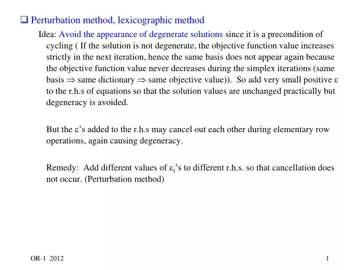
1. Perturbation method, lexicographic method Idea: Avoid the appearance of degenerate solutions since it is a precondition of cycling ( If the solution is not degenerate, the objective function value increases strictly in the next iteration, hence the same basis does not appear again because the objective function value never decreases during the simplex iterations (same basis  same dictionary  same objective value)). So add very small positive  to the r.h.s of equations so that the solution values are unchanged practically but degeneracy is avoided. But the ’s added to the r.h.s may cancel out each other during elementary row operations, again causing degeneracy. Remedy: Add different values of i’s to different r.h.s. so that cancellation does not occur. (Perturbation method)

2. Add to the r.h.s., with the following property. (3.4) • Then, it can be shown that the values of the basic variables never become 0 in subsequent simplex iterations, hence no cycling occurs. (In practice, precision can cause problems.) (In actual implementation, 1= , 2= 2, 3= 3, … may be used or random numbers in [0, ] for some fixed small  are used. )

3. (after two iterations, optimal solution obtained) Perturbation Method (tableau form) (0+21 ) (0+22 ) (1+3 )

4. Note that we can obtain the optimal solution and optimal value correctly after disregarding terms. The coefficients of do not affect the coefficients of other variables. • Perturbation method usually refers to the method which actually adds small to the right hand sides during simplex iterations. For lexicographic method, the idea is the same as the perturbation method. But we do not actually add some positive numbers to the r.h.s., but treat as symbols representing indefinite quantities, which satisfy (3.4).

5. Lexicographic ordering of numbers : Consider r = r0 + r1 1 + …. + rmm, s = s0 + s1 1 + …. + smm If r  s, there is the smallest subscript k such that rk  sk. We say that r is lexicographically smaller than s if rk < sk. (Similar terminology is used for vectors too) Then if , is lexicographically smaller than if and only if is numerically smaller than . • Ex)r = 2 + 211 + 19 2 + 200003 s = 2 + 211 + 202 + 203 + 154 + 145 is lexicographically smaller than .

6. Can cycling be prevented? • Thm 3.2: The simplex method terminates as long as the leaving variable is selected by the lexicographic rule in each iteration. Pf) see the proof in the text. For an arbitrary row with r.h.s. value , the proof shows that at least one of is distinct from zero. Hence no degenerate solution appears. • We may consider somewhat different logic to prove the result. The coefficient matrix for  variables in the constraints remain nonsingular after applying elementary row operations. (Elementary row operation is equivalent to premultiplying the corresponding nonsingular matrix to the coefficient matrix of constraints. Since the matrix for  variables is identity matrix initially, it is nonsingular. Hence we also obtain nonsingular coefficient matrix after elementary row operations are performed to the constraint matrix). In other words, no row with all 0 elements appear in the -matrix. Hence the values of basic variables never become 0 in lexicographic sense.

7. We can read the real solution value by ignoring the  terms in the current dictionary (tableau). It is also observed that the lexicographic method can be started and stopped at any time during the simplex iterations. We just add or drop the  terms at any time and it does not affect the real solution value and the coefficients of other variables in the tableau.

8. Practical Implementation of the Lexicographic Method • In real implementation of the lexicographic method, we do not actually add  terms to the r.h.s., but read the coefficients of  terms from the coefficients of other variables. • Note that, in the example, the coefficient matrix for the basic variables x5, x6, x7 and the coefficient matrix for 1, 2, 3 are the same identity matrices in the beginning of the lexicographic method. • Since we use the elementary row operations in the simplex pivots, those two coefficient matrices have the same elements in the following iterations. Hence, we can read the coefficients of 1, 2, 3 from the coefficients of x5, x6, x7 . So we do not actually need to add 1, 2, 3 to the tableau.

9. Hence, in the example, we actually do not need to add . We first perform ratio test using the entering column and the r.h.s. If ties occur, then perform ratio test (only for tied rows) again using the entering column and the column for , and then the column for , and then for , until tie is broken (lexicographic comparison of numbers).

10. (after two iterations) Example of real implementation (0+21 ) (0+22 ) (1+3 ) (after two iterations, optimal solution obtained)

11. Initialization (two-phase method) • We need an initial b.f.s to start the simplex method. • If we have for some constraint , the value of the slack variable violates nonnegativitiy constraint. maximize subject to , (1) Consider easily obtained solution for all in (1) and then subtract some positive number from all left-hand sides so that it becomes feasible solution to (1), i.e. for all , . Now, if we can find a feasible solution to (1) with , it is a feasible solution to (1) using original variables.

12. Hence solve the following problem using the easily obtained initial feasible solution and simplex method to find an optimal solution with . Note that x0 is a nonnegative variable. maximize (min ) subject to , (2) • (1) has a feasible solution  (2) has an optimal solution with optimal value 0 () • If we find an optimal solution with , we can obtain a feasible solution to (1) by disregarding . One point to be careful is that we need a basic feasible solution to perform the simplex method subsequently.

13. Example We cannot perform simplex iteration in this dictionary since the basic solution is not feasible (nonnegativity violated) However a feasible dictionary can be easily obtained by one pivot.

14. Current basic solution is not feasible. Let enter basis and the slack variable with most negative value leaves the basis (It is not a simplex iteration. Just perform the pivot, not considering the objective value. It does not change the solution set.) Perform simplex method. After two iterations, we get the optimal dictionary

15. We obtained optimal solution with value 0. Hence the current optimal solution gives a b.f.s. to the original problem. Drop (no more needed) and replace the objective function with the original one. z-row is used to read the objective value of a given solution, hence it can be added or dropped without affecting the feasible solution set to the LP. Note that the current b.f.s. is a b.f.s. to the original problem (We don’t have as a basic variable).

16. Express it in dictionary form (only nonbasic variables appear in the r.h.s.) by substituting the basic variables in the objective function. Now, restart the simplex method with the current dictionary

17. You need to understand that (i) can be added or dropped from the dictionary, but the set of feasible solutions to LP (disregarding variable ) doesn’t change since the coefficients of in the dictionary don’t affect the coefficients of other variables as long as we perform elementary row operations (simplex pivots). The additional variable is used temporarily for the purpose of identifying a basic feasible solution to the original problem. Once the value of becomes 0 (as a nonbasic variable), can be eliminated without affecting the values of the current solution. Also (ii) the objective row can be exchanged by another objective row at any time, but the set of feasible solutions to LP doesn’t change because the set of feasible solutions to LP has not been affected by the objective row during the simplex pivots. • See the next slides for the two phase method, which are expressed with tableau format.

18. tableau form -w -x0 = 0 2x1 - x2 + 2x3 - x0 + x4 = 4 2x1 - 3x2 + x3 - x0 + x5 = -5 -x1 + x2 - 2x3 - x0 + x6 = -1 -w -2x1 + 3x2 - x3 - x5= -5 2x2 + x3 + x4- x5 = 9 -2x1 + 3x2 - x3 + x0 - x5 = 5 -3x1 + 4x2 - 3x3 - x5 + x6 = 4 elmentary row operations -w - x0= 0 0.2x1+ x3 +0.8x0 - 0.2x5 - 0.6x6 = 1.6 -0.6x1 + x2 +0.6x0 - 0.4x5 - 0.2x6 = 2.2 x1 -2x0 + x4 + x6 = 3

19. Note that the coefficients of x0 do not affect the coefficients of other variables in the simplex pivots. • Suppose we perform the same pivots, disregarding variable x0. Then we obtain the same final tableau without x0. • The 3 constraints in the initial tableau without variable x0defines feasible solution set of the augmented LP (with nonnegativity of variables) • Therefore, the final tableau (without x0) describes the same feasible solution set of the LP, i.e. feasible solutions to the equations have not changed. • Now, we can replace the objective function with the original one, and express it in the formal tableau form. -w - x0= 0 0.2x1+ x3 +0.8x0 - 0.2x5 - 0.6x6 = 1.6 -0.6x1 + x2 +0.6x0 - 0.4x5 - 0.2x6 = 2.2 x1 -2x0 + x4 + x6 = 3 -z + x1 - x2 + x3= 0 0.2x1+ x3- 0.2x5 - 0.6x6 = 1.6 -0.6x1 + x2 - 0.4x5 - 0.2x6 = 2.2 x1 + x4 + x6 = 3 -z + 0.2x1 - 0.2x5 + 0.4x6= 0.6 0.2x1+ x3- 0.2x5 - 0.6x6 = 1.6 -0.6x1 + x2 - 0.4x5 - 0.2x6 = 2.2 x1 + x4 + x6 = 3

20. Algorithm strategy in phase one: choose as leaving variable in case of ties in the minimum ratio test. • 2 possible cases in phase one optimal solution • nonzero ( ), basic  original problem is infeasible • nonbasic drop , express original objective function in terms of nonbasic variables, continue the simplex method. (Note that basic can’t happen by our strategy) • Similar idea can be used when the original LP is given in equality form and we do not have an initial basic feasible solution at hand. (Without replacing an equality with two inequalities, simplex method can be used directly to solve the equality form. More in Chapter 8.)

21. (Fundamental theorem of LP) Every LP in standard form has the following properties. • If no optimal solution  either unbounded or infeasible. • If  feasible solution   a basic feasible solution. • If  optimal solution   a basic optimal solution.