Introduction

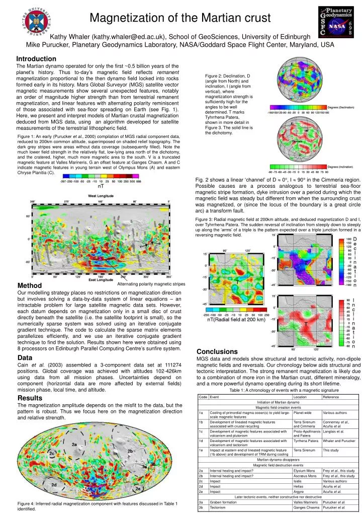
1. Magnetization of the Martian crustKathy Whaler (kathy.whaler@ed.ac.uk), School of GeoSciences, University of EdinburghMike Purucker, Planetary Geodynamics Laboratory, NASA/Goddard Space Flight Center, Maryland, USA Introduction The Martian dynamo operated for only the first ~0.5 billion years of the planet’s history. Thus to-day’s magnetic field reflects remanent magnetization proportional to the then dynamo field locked into rocks formed early in its history. Mars Global Surveyor (MGS) satellite vector magnetic measurements show several unexpected features, notably an order of magnitude higher strength than from terrestrial remanent magnetization, and linear features with alternating polarity reminiscent of those associated with sea-floor spreading on Earth (see Fig. 1). Here, we present and interpret models of Martian crustal magnetization deduced from MGS data, using an algorithm developed for satellite measurements of the terrestrial lithospheric field. Figure 2: Declination, D (angle from North) and inclination, I (angle from vertical), where magnetization strength is sufficiently high for the angles to be well determined. T marks Tyhrrhena Patera, shown in more detail in Figure 3. The solid line is the dichotomy. Figure 1: An early (Purucker et al., 2000) compilation of MGS radial component data, reduced to 200km common altitude, superimposed on shaded relief topography. The dark grey stripes were areas without data coverage (subsequently filled). Note the much lower field strength in the relatively flat, low-lying area north of the dichotomy, and the cratered, higher, much more magnetic area to the south. V is a truncated magnetic feature at Valles Marineris, G an offset feature at Ganges Chasm. A and C indicate magnetic features in young terrain west of Olympus Mons (A) and eastern Chryse Planitia (C). Fig. 2 shows a linear ‘channel’ of D  0°, I  90° in the Cimmeria region. Possible causes are a process analogous to terrestrial sea-floor magnetic stripe formation, dyke intrusion over a period during which the magnetic field was steady but different from when the surrounding crust was magnetized, or (since the locus of the boundary is a great circle arc) a transform fault. Figure 3: Radial magnetic field at 200km altitude, and deduced magnetization D and I, over Tyhrrhena Patera. The sudden reversal of inclination from steeply down to steeply up along the ‘arms’ of a triple is the pattern expected over a triple junction formed in a reversing magnetic field. Method Our modelling strategy places no restrictions on magnetization direction but involves solving a data-by-data system of linear equations – an intractable problem for large satellite magnetic data sets. However, each datum depends on magnetization only in a small disc of crust directly beneath the satellite (i.e. the satellite footprint is small), so the numerically sparse system was solved using an iterative conjugate gradient technique. The code to calculate the sparse matrix elements parallelizes efficiently, and we use an iterative conjugate gradient technique to find the solution. Results shown here were obtained using 8 processors on Edinburgh Parallel Computing Centre’s sunfire system. Alternating polarity magnetic stripes Conclusions MGS data and models show structural and tectonic activity, non-dipole magnetic fields and reversals. Our chronology below aids structural and tectonic interpretation. The strong remanent magnetization is likely due to a combination of more iron in the Martian crust, different mineralogy, and a more powerful dynamo operating during its short lifetime. Data Cain et al. (2003) assembled a 3-component data set at 111274 positions. Global coverage was achieved with altitudes 102-426km using data from all mission phases. Uncertainties depend on component (horizontal data are more affected by external fields) mission phase, local time, and altitude. Table 1: A chronology of events with a magnetic signature Results The magnetization amplitude depends on the misfit to the data, but the pattern is robust. Thus we focus here on the magnetization direction and relative strength. Figure 4: Inferred radial magnetization component with features discussed in Table 1 identified.