Download
1 / 22

E N D
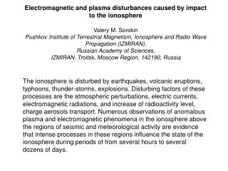
International EU-Russia/CIS Conference on technologies of the future: Spain-ISTC/STCU cooperation. Madrid, 22-23 April 2010An Event under the Spanish Presidency of the EUAerospace monitoring of natural and technological disasters V.M. Sorokin and V.M. ChmyrevPushkov Institute of Terrestrial Magnetism, Ionosphere and Radio Wave Propagation, Russian Academy of Sciences (IZMIRAN), 142190 Troitsk, Moscow region, Russian FederationSchmidt Institute of Physics of the Earth (IPE), Russian Academy of Sciences, 10B, Gruzinskaya Str., 123995 Moscow, Russian Federation This report presents the methods for monitoring of large-scale natural and technological disasters. The methods are based on the latest achievements in study of the seismo-ionospheric coupling and the formation mechanisms of the disturbances in near Earth space at the preparatory phases of earthquakes.
Basic experimental results. • Enhancement of seismic activity and typhoons produce DC electric field disturbances in the ionosphere of the order of 10 mV/m. • These ionospheric disturbances occupy the region of the order of several hundred km in diameter over epicenter. • DC electric field enhancements arise in the ionosphere from hours to 10 days before earthquakes. • Within the seismically disturbed geomagnetic field tube the small scale (~10 km) irregularities of plasma density with relative amplitude ~10 % are observed together with the magnetic field disturbances ~10 nT and the electromagnetic emissions in ELF range with amplitude ~10 pT. • DC electric field on the Earth surface in epicenter area does not exceed the background value ~100 V/m.
The key role in the seismo-ionospheric interaction belongs to external currents in the lower atmosphere. The external current is excited in a process of vertical atmospheric convection and gravitational sedimentation of charged aerosols. Aerosols are injected into the atmosphere due to intensifying soil gas elevation in the lithosphere during the enhancement of seismic activity. Its inclusion into the atmosphere – ionosphere electric circuit leads to DC electric field growth up to 10 mV/m in the lower ionosphere.
The proposed methods for monitoring of seismic activity are based on the electrodynamic model of the atmosphere – ionosphere coupling 1. Earth surface 2. Conductive layer of the ionosphere 3. External electric current in the lower atmosphere 4. Conductivity electric current in the atmosphere – ionosphere circuit 5. Geomagnetic field - aligned electric current in the ionosphere 6. Satellite trajectory 7. Charged aerosols injected into the atmosphere by soil gases
Calculation results of the altitude dependences of atmosphere conductivity at the epicenter of disturbed region.Left panel shows the atmosphere conductivity at different levels of atmospheric radioactivity. Right panel presents the atmosphere conductivity at different number density of charged aerosols over the Earth’s surface.
The altitude dependences of external electric current at the epicenter of disturbed region. • External current is formed as a result of: • convective transfer of charged aerosols, • ionization of lower atmosphere by radioactive sources, • adhesion of electrons to molecules, • interaction of charged ions with charged aerosols
DC electric field calculated for axially symmetric distribution of the external electric current Upper panel: Horizontal DC electric field in the ionosphere along and across the plane of the geomagnetic meridian. Angle of the magnetic field inclination is Middle panel: Vertical component of DC electric field on the Earth surface. Lower panel: Normalized vertical component of the external current on the Earth surface.
Spatial distributions of DC electric field calculated for axially symmetric distribution of the external electric current Upper panel: Horizontal component of DC electric field in the ionosphere. Angle of themagnetic field inclination is Lower panel: Vertical component of DC electric field on the ground.
Spatial distribution of horizontal component of the electric field in the ionosphere and of vertical component of the electric field on the Earth surface over the fault in a form of ellipse.
Model examples of the altitude electric field distribution in the Earth – ionosphere layer (in relative units).
Formation of field-aligned currents and plasma irregularities in the upper ionosphere as a result of Acoustic Gravity Wave (AGW) instability in the lower ionosphere. The excitation of horizontal spatial structure of conductivity in the lower ionosphere results in the formation of magnetic field- aligned currents and plasma layers stretched along the geomagnetic field.
Examples of satellite observations of ULF magnetic field oscillations, electron number density fluctuations and ELF electromagnetic emissions caused by the formation of the ionosphere conductivity irregularities. 1. Earthquake. 2. Irregularities of ionosphere conductivity. 3. Field-aligned currents and irregularities of electron number density. 4. Satellite trajectory crossing the disturbed region. ULF magnetic field. Electron number density fluctuations. ELF electromagnetic emissions
The excitation of horizontal small-scale irregularities of electric conductivity in the lower ionosphere can be used as a basis for thegeneration mechanism of electromagnetic ELF precursors to earthquakes. These waves are generated in a process of interaction of thunderstorm related EM radiation with small-scale plasma irregularities excited in the lower ionosphere before earthquakes. These EM pulses are radiated by lightning discharges and propagate in the sub-ionospheric wave guide with small attenuation in ELF range
Spatial distribution of electron number density in the ionosphic E - region caused by the electric current flowing into the ionosphere from the atmosphere.
Spatial distribution of electron number density in the D layer of the ionosphere caused by the electric current flowing from the atmosphere to the ionosphere
The scheme of processes responsible for the atmosphere – ionosphere coupling
Composition of the Combined Space, Airborne and Ground-Based Short – Term Earthquake Forecasting System Space segment Aviation segment Ground segment Small satellite grouping M-55 “GEOPHYSICS” stratospheric aircraft Network of geophysical stations Microsatellite grouping Ground Control Complex & Data Processing and Analysis Center g and Analysis Center
The satellite segment of the monitoring system should provide the measurements of the following field and plasma parameters: • Three components of DC electric field; • Electromagnetic field waveforms; • Spectral density for wave components; • Thermal plasma parameters - components of ion drift velocity, ion number density, ion temperature, ion density oscillations; • Intensity of IR radiation for mapping thermal anomalies; • Limb measurements of the spectral distribution of hydroxyl emission; • Thunderstorm activity.
Aviation segment based on the stratospheric M-55 “Geophysics” aircraft Atmosphere monitoring at the altitudes up to 21 km Earth multi-spectral remote sensing with coverage up to 120 km The basic performance: • Range of flight altitudes : 0 – 21 km; • Max payload: 2000 kg; • Speed range at 20 km altitude: 660 – 740 km/h; • Flight time: 6 hours; • Required runway length: 1800 m; • Equipment power supply: 40 kW of AC 115/200 V 400 Hz combined with 3 kW DC 27 V; • Power plant: 2 turbofan PS 30V12; • Non-pressurized dust-moisture-proof bays with 9 cubic meters total volume enabling installation of equipment operating independently through top, side and down-view windows. The measured parameters: • Composition and spatial distribution of aerosols; • Chemical and isotope composition of the atmosphere; • Atmospheric optical emissions; • DC electric and magnetic fields; • ULF/ELF/VLF electromagnetic radiation; • Intensity of IR radiation; • Multi-spectral images
GROUND GEOPHYSICAL SEGMENT EACH STATION IS EQUIPPED WITH INSTRUMENTS FOR CONTINUOS MEASUREMENTS OF • SEISMIC AND MAGNETIC FIELD OSCILLATIONS, • NATURAL ULF/ELF/VLF ELECTROMAGNETIC EMISSIONS AND VLF/LF TRANSMITTER SIGNALS, • ATMOSHERIC DC ELECTRIC FIELDS AND TELLURIC CURRENTS, • CHEMICAL COMPOSITION OF SOIL, WATERS, AND ATMOSPHERIC GAS, • AEROSOL CHARACTERISTICS, • RADON AND OTHER RADIOACTIVE GAS EMISSIONS, • DISTURBANCES OF D, E, AND F LAYERS OF THE IONOSPHERE. ALL GEOPHYSICAL STATIONS ARE CONNECTED WITH GROUND CONTROL COMPLEX AND DATA PROCESSING CENTER.
G Kamchatkan volcanoes in Russia are practically always active and extremely hazardous to jet aircraft flying over North Pacific The Eyjafjallajokull volcano in Iceland, which was sleeping during more than 200 years now has woken and produced the aviation transport collapse in Europe. Is this a time for our governments to wake up and start investing in the disaster monitoring and prediction of catastrophes? THANKS .