Download
1 / 46
460 likes | 627 Views
Statistics for Microarrays. Normalization Review and Cluster Analysis. Class web site: http://statwww.epfl.ch/davison/teaching/Microarrays/. Normalization Methods. Global adjustment (e.g. median or mean for a set of genes)

E N D
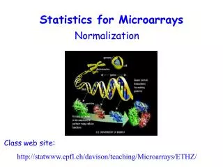
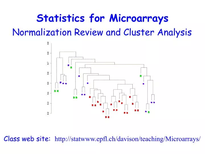
Statistics for Microarrays Normalization Review and Cluster Analysis Class web site: http://statwww.epfl.ch/davison/teaching/Microarrays/
Normalization Methods • Global adjustment (e.g. median or mean for a set of genes) • Intensity-dependent -- shift M by c=c(A); e.g. c(A) made with lowess • Within print-tip group normalization to correct for spatial bias • Both print-tip and intensity-dependent adjustment: perform LOWESS fits to the data within print-tip groups
Normalization: Which Spots to use? The LOWESS lines can be run through many different sets of points, and each strategy has its own implicit set of assumptions justifying its applicability. For example, the use of a global LOWESS approach can be justified by supposing that, when stratified by mRNA abundance, a) only a minority of genes are expected to be differentially expressed, or b) any differential expression is as likely to be up-regulation as down-regulation. Pin-group LOWESS requires stronger assumptions: that one of the above applies within each pin-group. The use of other sets of genes, e.g. control or housekeeping genes, involve similar assumptions.
Pre-processed cDNA Gene Expression Data Slides On p genes for n slides: p is O(10,000), n is O(10-100), but growing, slide 1 slide 2 slide 3 slide 4 slide 5 … 1 0.46 0.30 0.80 1.51 0.90 ... 2 -0.10 0.49 0.24 0.06 0.46 ... 3 0.15 0.74 0.04 0.10 0.20 ... 4 -0.45 -1.03 -0.79 -0.56 -0.32 ... 5 -0.06 1.06 1.35 1.09 -1.09 ... Genes Gene expression level of gene 5 in slide 4 = Log2(Red intensity / Green intensity) These values are conventionally displayed on a red(>0)yellow (0)green (<0) scale.
Cluster analysis • Used to find groups of objects when not already known • “Unsupervised learning” • Associated with each object is a set of measurements (the feature vector) • Aim is to identify groups of similar objects on the basis of the observed measurements
Clustering Gene Expression Data • Can cluster genes (rows), e.g. to (attempt to) identify groups of co-regulated genes • Can cluster samples (columns), e.g. to identify tumors based on profiles • Can cluster both rows and columns at the same time
Clustering Gene Expression Data • Leads to readily interpretable figures • Can be helpful for identifying patterns in time or space • Useful (essential?) when seeking new subclasses of samples • Can be used for exploratory purposes
Similarity • Similarity sij indicates the strength of relationship between two objects i and j • Usually 0 ≤ sij ≤1 • Correlation-based similarity ranges from –1 to 1
Dissimilarity and Distance • Associated withsimilarity measures sij bounded by 0 and 1 is a dissimilarity dij = 1 - sij • Distance measures have the metric property (dij +dik ≥ djk) • Many examples: Euclidean, Manhattan, etc. • Distance measure has a large effect on performance • Behavior of distance measure related to scale of measurement
Partitioning Methods • Partition the objects into a prespecified number of groups K • Iteratively reallocate objects to clusters until some criterion is met (e.g. minimize within cluster sums of squares) • Examples: k-means, partitioning around medoids (PAM), self-organizing maps (SOM), model-based clustering
Hierarchical Clustering • Produce a dendrogram • Avoid prespecification of the number of clusters K • The tree can be built in two distinct ways: • Bottom-up: agglomerative clustering • Top-down: divisive clustering
Agglomerative Methods • Start with n mRNA sample (or G gene) clusters • At each step, merge the two closest clusters using a measure of between-cluster dissimilarity which reflects the shape of the clusters • Examples of between-cluster dissimilarities: • Unweighted Pair Group Method with Arithmetic Mean (UPGMA): average of pairwise dissimilarities • Single-link (NN): minimum of pairwise dissimilarities • Complete-link (FN): maximum of pairwise dissimilarities
Divisive Methods • Start with only one cluster • At each step, split clusters into two parts • Advantage: Obtain the main structure of the data (i.e. focus on upper levels of dendrogram) • Disadvantage: Computational difficulties when considering all possible divisions into two groups
Partitioning vs. Hierarchical • Partitioning • Advantage: Provides clusters that satisfy some optimality criterion (approximately) • Disadvantages: Need initial K, long computation time • Hierarchical • Advantage: Fast computation (agglomerative) • Disadvantages: Rigid, cannot correct later for erroneous decisions made earlier
Generic Clustering Tasks • Estimating number of clusters • Assigning each object to a cluster • Assessing strength/confidence of cluster assignments for individual objects • Assessing cluster homogeneity
Bittner et al. It has been proposed (by many) that a cancer taxonomy can be identified from gene expression experiments.
Dataset description • 31 melanomas (from a variety of tissues/cell lines) • 7 controls • 8150 cDNAs • 6971 unique genes • 3613 genes ‘strongly detected’
Average linkage hierarchical clustering, melanoma only 1-r = .54 unclustered ‘cluster’
Issues in Clustering • Pre-processing (Image analysis and Normalization) • Which genes (variables) are used • Which samples are used • Which distance measure is used • Which algorithm is applied • How to decide the number of clusters K
Issues in Clustering • Pre-processing (Image analysis and Normalization) • Which genes (variables) are used • Which samples are used • Which distance measure is used • Which algorithm is applied • How to decide the number of clusters K
Filtering Genes • All genes (i.e. don’t filter any) • At least k (or a proportion p) of the samples must have expression values larger than some specified amount, A • Genes showing “sufficient” variation • a gap of size A in the central portion of the data • a interquartile range of at least B • Filter based on statistical comparison • t-test • ANOVA • Cox model, etc.
Issues in Clustering • Pre-processing (Image analysis and Normalization) • Which genes (variables) are used • Which samples are used • Which distance measure is used • Which algorithm is applied • How to decide the number of clusters K
Average linkage hierarchical clustering, melanoma only unclustered ‘cluster’
Average linkage hierarchical clustering, melanoma & controls unclustered ‘cluster’ control
Issues in clustering • Pre-processing • Which genes (variables) are used • Which samples are used • Which distance measure is used • Which algorithm is applied • How to decide the number of clusters K
Issues in clustering • Pre-processing • Which genes (variables) are used • Which samples are used • Which distance measure is used • Which algorithm is applied • How to decide the number of clusters K
Issues in clustering • Pre-processing • Which genes (variables) are used • Which samples are used • Which distance measure is used • Which algorithm is applied • How to decide the number of clusters K
How many clusters K? • Many suggestions for how to decide this! • Milligan and Cooper (Psychometrika 50:159-179, 1985) studied 30 methods • Some new methods include GAP (Tibshirani ) and clest (Fridlyand and Dudoit) • Applying several methods yielded estimates of K = 2 (largest cluster has 27 members) to K = 8 (largest cluster has 19 members)
Average linkage hierarchical clustering, melanoma only unclustered cluster
Summary • Buyer beware – results of cluster analysis should be treated with GREAT CAUTION and ATTENTION TO SPECIFICS, because… • Many things can vary in a cluster analysis • If covariates/group labels are known, then clustering is usually inefficient
IPAM Group, UCLA: Debashis Ghosh Erin Conlon Dirk Holste Steve Horvath Lei Li Henry Lu Eduardo Neves Marcia Salzano Xianghong Zhao Others: Sandrine Dudoit Jane Fridlyand Jose Correa Terry Speed William Lemon Fred Wright Acknowledgements