Statistics for Microarrays
480 likes | 686 Views
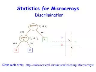
Statistics for Microarrays. Experimental Design and Differential Expression. Class web site: http://statwww.epfl.ch/davison/teaching/Microarrays/ETHZ/. Biological question Differentially expressed genes Sample class prediction etc. Experimental design. Microarray experiment.

Statistics for Microarrays
E N D
Presentation Transcript
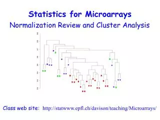
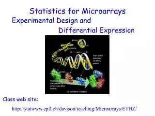
Statistics for Microarrays Experimental Design and Differential Expression Class web site: http://statwww.epfl.ch/davison/teaching/Microarrays/ETHZ/
Biological question Differentially expressed genes Sample class prediction etc. Experimental design Microarray experiment 16-bit TIFF files Image analysis (Rfg, Rbg), (Gfg, Gbg) Normalization R, G Estimation Testing Clustering Discrimination Biological verification and interpretation
Some Considerations for cDNA Microarray Experiments (I) • Scientific (Aims of the experiment) • Specific questions and priorities • How will the experiments answer the questions • Practical (Logistic) • Types of mRNA samples: reference, control, treatment, mutant, etc • Source and Amount of material (tissues, cell lines) • Number of slides available
Some Considerations for cDNA Microarray Experiments (II) • Other Information • Experimental process prior to hybridization: sample isolation, mRNA extraction, amplification, labelling,… • Controls planned: positive, negative, ratio, etc. • Verification method: Northern, RT-PCR, in situ hybridization, etc.
Aspects of Experimental Design Applied to Microarrays (I) Array Layout • Which cDNA sequences are printed • Spatial position Allocation of samples to slides • Design layouts • A vs B: Treatment vs control • Multiple treatments • Factorial • Time series
Aspects of Experimental Design Applied to Microarrays (II) Other considerations • Replication • Physical limitations: the number of slides and the amount of material • Sample Size • Extensibility - linking
Layout options The main issue is the use of reference samples, typically labelled green. Standard statistical design principles can lead to more efficient layouts; use of dye-swaps can also help. Sample size determination is more than usually difficult, as there are 1,000s of possible changes, each with its own SD.
Case 1: Meaningful biological control (C) Samples: Liver tissue from four mice treated by cholesterol modifying drugs. Question 1: Genes that respond differently between the T and the C. Question 2: Genes that responded similarly across two or more treatments relative to control. Case 2: Use of universal reference Samples: Different tumor samples. Question: To discover tumor subtypes. T2 T3 T4 T1 T2 Tn Tn-1 T1 Ref Natural design choice C
Treatment vs Control Two samples e.g. KO vs. WT or mutant vs. WT Indirect Direct T Ref T C C Ref average (log (T/C)) log (T / Ref) – log (C / Ref ) 2 /2 22
A B C A A B C C B ref ref One-way layout: one factor, k levels
A B C A A B C C B ref ref One-way layout: one factor, k levels For k = 3, efficiency ratio (Design I / Design III) = 3. In general, efficiency ratio = 2k / (k-1). (But may not be achievable due to lack of independence.)
A B C Illustration from one experiment Design I A B C Ref Design III Box plots of log ratios: direct still ahead
Factorial experiments • Treated cell lines • Possible experiments OSM CTL OSM &EGF EGF Here interest is not in genes for which there is anO or an E (main) effect, but in which there is an OEinteraction, i.e. in genes for which log(O&E/O)-log(E/C) is large or small.
C A C A C A A B A.B A.B A.B B B A.B B C 2 x 2 factorial: some design options Table entry: variance (assuming all log ratios uncorrelated)
Some Design Possibilities for Detecting Interaction Samples: treated tumor cell lines at 4 time points (30 minutes, 1 hour, 4 hours, 24 hours) Question: Which genes contribute to the enhanced inhibitory effect of OSM when it is combined with EGF? Role of time? Design A: Design B: ctl ctl OSM 2 OSM & EGF OSM & EGF EGF OSM EGF
Combining Estimates D A Different ways of estimating the same contrast: e.g. A compared to P Direct = A-P Indirect = A-M + (M-P) or A-D + (D-P) or -(L-A) - (P-L) M L P V How do we combine these?
Time Course Experiments • Number of time points • Which differences are of highest interest (e.g. between initial time and later times, between adjacent times) • Number of slides available
T2 T4 T1 T3 T2 T4 T1 T3 T2 T4 T1 T3 Ref T1 T2 T3 T4 T1 T2 T3 T4 T2 T4 T1 T3
Replication • Why? • To reduce variability • To increase generalizability • What is it? • Duplicate spots • Duplicate slides • Technical replicates • Biological replicates
Technical Replicates: Labeling • 3 sets of self – self hybridizations • Data 1 and Data 2 were labeled together and hybridized on two slides separately • Data 3 were labeled separately Data 3 Data 2 Data 1 Data 1
Sample Size • Variance of individual measurements (X) • Effect size(s) to be detected (X) • Acceptable false positive rate • Desired power (probability of detecting an effect of at least the specfied size)
Extensibility • “Universal” common reference for arbitrary undetermined number of (future) experiments • Provides extensibility of the series of experiments (within and between labs) • Linking experiments necessary if common reference source diminished/depleted
Summary • Balance of direct and indirect comparisons • Optimize precision of the estimates among comparisons of interest • Must satisfy scientific and physicalconstraints of the experiment
Identifying Differentially Expressed Genes • Goal: Identify genes associated with covariate or response of interest • Examples: • Qualitative covariates or factors: treatment, cell type, tumor class • Quantitative covariate: dose, time • Responses: survival, cholesterol level • Any combination of these!
Biological question Differentially expressed genes Sample class prediction etc. Experimental design Microarray experiment 16-bit TIFF files Image analysis (Rfg, Rbg), (Gfg, Gbg) Normalization R, G Estimation Testing Clustering Discrimination Biological verification and interpretation
Differentially Expressed Genes • Simultaneously test m null hypotheses, one for each gene j : Hj: no association between expression level of gene j and covariate/response • Combine expression data from different slides and estimate effects of interest • Compute test statistic Tj for each gene j • Adjust for multiple hypothesis testing
Test statistics • Qualitative covariates: e.g. two-sample t-statistic, Mann-Whitney statistic, F-statistic • Quantitative covariates: e.g. standardized regression coefficient • Survival response: e.g. score statistic for Cox model
Example: Apo AI experiment(Callow et al., Genome Research, 2000) GOAL: Identify genes with altered expression in the livers of one line of mice with very low HDL cholesterol levels compared to inbred control mice Experiment: • Apo AI knock-out mouse model • 8 knockout (ko) mice and 8 control (ctl) mice (C57Bl/6) • 16 hybridisations: mRNA from each of the 16 mice is labelled with Cy5, pooled mRNA from control mice is labelled with Cy3 Probes: ~6,000 cDNAs, including 200 related to lipid metabolism
Which genes have changed? This method can be used with replicated data: 1. For each gene and each hybridisation (8 ko + 8 ctl) use M=log2(R/G) 2. For each gene form the t-statistic: average of 8 ko Ms - average of 8 ctl Ms sqrt(1/8 (SD of 8 ko Ms)2 + 1/8 (SD of 8 ctl Ms)2) 3. Form a histogram of 6,000 t values 4. Make a normal Q-Q plot; look for values “off the line” 5. Adjust for multiple testing
Histogram & Q-Q plot ApoA1
Assigning p-values to measures of change • Estimate p-values for each comparison (gene) by using the permutation distribution of the t-statistics. • For each of the possible permutation of the trt / ctl labels, compute the two-sample t-statistics t* for each gene. • The unadjusted p-value for a particular gene is estimated by the proportion of t*’s greater than the observed t in absolute value.
Apo AI: Adjusted and unadjusted p-values for the 50 genes with the larges absolute t-statistics
Single-slide methods • Model-dependent rules for deciding whether (R,G) corresponds to a differentially expressed gene • Amounts to drawing two curves in the (R,G)-plane; call a gene differentially expressed if it falls outside the region between the two curves • At this time, not enough known about the systematic and random variation within a microarray experiment to justify these strong modeling assumptions • n = 1 slide may not be enough (!)
Single-slide methods • Chen et al: Each (R,G) is assumed to be normally and independently distributed with constant CV; decision based on R/G only (purple) • Newton et al: Gamma-Gamma-Bernoulli hierarchical model for each (R,G) (yellow) • Roberts et al: Each (R,G) is assumed to be normally and independently distributed with variance depending linearly on the mean • Sapir & Churchill: Each log R/G assumed to be distributed according to a mixture of normal and uniform distributions; decision based on R/G only (turquoise)
Difficulty in assigning valid p-values based on a single slide Matt Callow’s Srb1 dataset (#8). Newton’s, Sapir & Churchill’s and Chen’s single slide method
Another example: Survival analysis with expression data • Bittner et al. looked at differences in survival between the two groups (the ‘cluster’ and the ‘unclustered’ samples) • ‘Cluster’ seemed to have longer survival
Average Linkage Hierarchical Clustering, survival only unclustered cluster
Identification of genes associated with survival For each gene j, j = 1, …, 3613, model the instantaneous failure rate, or hazard function, h(t) with the Cox proportional hazards model: h(t) = h0(t)exp(jxij) • and look for genes with both: • large effect size j • large standardized effect size j/SE(j) ^ ^ ^
Findings • Top 5 genes by this method not in Bittner et al. ‘weighted gene list’ - Why? • weighted gene list based on entire sample; our method only used half • weighting relies on Bittner et al. cluster assignment • other possibilities?
Limitations of Single Gene Tests • May be too noisy in general to show much • Do not reveal coordinated effects of positively correlated genes • Hard to relate to pathways
Some ideas for further work • Expand models to include more genes and possibly two-way interactions • Nonparametric tree-based subset selection – would require much larger sample sizes
Acknowledgements • Sandrine Dudoit • Jane Fridlyand • Yee Hwa (Jean) Yang • Debashis Ghosh • Erin Conlon • Ingrid Lonnstedt • Terry Speed