Download
1 / 21
250 likes | 711 Views
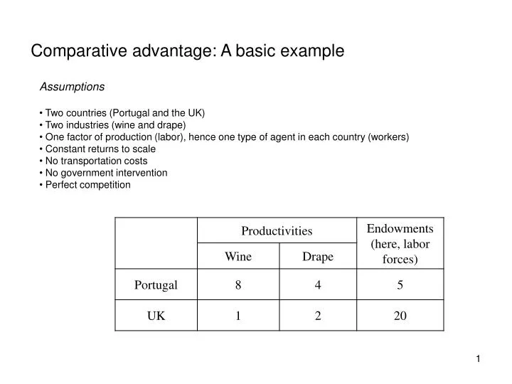
Comparative advantage: A basic example. Assumptions Two countries (Portugal and the UK) Two industries (wine and drape) One factor of production (labor), hence one type of agent in each country (workers) Constant returns to scale No transportation costs No government intervention

E N D
Comparative advantage: A basic example • Assumptions • Two countries (Portugal and the UK) • Two industries (wine and drape) • One factor of production (labor), hence one type of agent in each country (workers) • Constant returns to scale • No transportation costs • No government intervention • Perfect competition
Portugal’s production-possibility frontier and the autarky (before-trade) equilibrium Wine Consumer preferences (demand side) 40 Consumption point without international trade Production possibility frontier (supply side) Drape 20
The UK’s production-possibility frontierand the autarky equilibrium Wine Production possibility frontier (supply side) Consumption point without international trade 20 Indifference curve (demand curve)) Drape 40
The world’s production-possibility frontierand trading equilibrium World production possibility frontier Wine world price ratio (demand-determined) United Kingdom Consumer preferences (common to all countries) 40 Consumption point with international trade Portugal Drape 40
The gains from exchange revisited Wine Indifference curves Production Possibility Frontier world price ratio Drape
The gains from specialization Wine Production point Indifference curves world price ratio Production Possibility Frontier Drape
The Rybszinski theorem steel production possibility frontier after an increase in the capital endowment initial production possibility frontier production possibility frontier after an increase in the labor endowment drape
The Heckscher-Ohlin theorem (world & domestic) indifference curves steel world price ratio (drape is cheaper) home steel exports “trade triangle” domestic PPF drape home drape imports domestic price ratio (before trade)
P S* P S P*a Pa D* D Country H (relatively efficient) Country F (relatively inefficient) The gains from trade (i): initial equilibrium Quantities
Equilibrium price Method 1: Equate segments ab and cd P P* Country H Country F P*a a b Pw c d Pa
Equilibrium price Method 2 a) Construct excess supply (ES) and excess demand (ED) curves Home ES ab = cd a b c d Pa Export supply Pa* ab = cd a b c d Foreign ED* Import demand
Equilibrium price, method 2 b) Match the home ES and foreign ED curves on single « world » market S* Pa* ES P*a S Pw D* Pa ED* D Quantities E=M* Country H (exporter) Country F (importer) « World » market
Gains from goods trade Importer country consumers’ gain, producers’ loss = neutral P A B K C pa F J p* World price G H I D ED (a) Importer country’s domestic market (b) same thing seen on world market
Gains from goods trade Exporter country producers’ gain, consumers’ loss = neutral A ES F p* E H G D World price B C I pa EF (a) Exporter country’s domestic market (b) same thing seen on world market
Who gains from trade Size and « similarity » More « different » exporter gains more from trade ES ES Net increase in importer country’s welfare = CS gain – PS loss SIMILARITY ED ED ES ED Larger exporter gains less from trade ES Net increase in exporter country’s welfare = PS gain – CS loss SIZE ES ED ED
Value of marginal product of capital r Economy’s capital stock Return to other factors ra Return to capital + = GDP (equal to GNP in autarky) K Gains from factors trade Starting point: autarky Very similar to trade in G&S: Identical causes: differences in prices (factor rewards) Identical consequences: some gains, other loose, and there is a net potential gain.
Gains from factors trade Capital flow from Home to Foreign Two countries, H relatively well endowed with capital. Initially, rH < rF, so capital has an incentive to migrate from H to F VF = p*F*K VH = pFK In equilibrium, the marginal products of capital are equalized. Gains from capital movements: EBCfor H, EIBfor F. A I rF E rW B D G C rH Home capital stock (before outflow) Foreign capital stock (before inflow) Extension of foreign capital stock (because of inflow)
Home country’s GDP Foreign country’s GDP Gains from factors trade GNP vs. GDP, efficiency gain VF=p*F*K VH=pFK GNP GNP* Efficiency gain from capital flow
Openness and size Trade share in GDP Larger countries trade less (not so obvious) Not very open given their size (should trade more) GDP at purchasing power parity
Transportation costs “Fob”: free-on-board; “cif”: cum insurance and freight. Transport cost per unit: Pcif = Pfob + = Pa + Condition for trade to take place: Pa + Pa* If condition violated, good is said to be non-traded EScif P*a ESfob Pwcif Pwfob ED* Pa Less trade