Query Processing and Optimization
220 likes | 417 Views
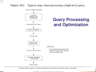
Query Processing and Optimization. One View of Basic Query Processing Steps. Another View of Basic Query Processing Steps. Example of a Bind Variable: select * from emp where sal = :salary. Another View of Basic Query Processing Steps.

Query Processing and Optimization
E N D
Presentation Transcript
One View of Basic Query Processing Steps Data Management
Another View of Basic Query Processing Steps Example of a Bind Variable: select * from emp where sal = :salary Data Management
Another View of Basic Query Processing Steps Data Management
Before showing query processing examples, we need to discuss some Oracle Join Methods. Nested loops join The nested loop iterates over all rows of the outer table. If there are conditions in the where clause of the SQL statement that apply to the outer table only, it checks whether those apply. If they do, the corresponding rows (from the where condition) in the joined inner table are searched. These rows from the inner table are either found using an index (if a suitable index exists) or by doing a full table scan. Merge join (also called sort merge join) A merge join basically sorts all relevant rows in the first table by the join key , and also sorts the relevant rows in the second table by the join key, and then merges these sorted rows. Take an example! At a garage sale you can buy 400 books. The deal is to take all or none. You take all. Now, you have to find the books that you already have at home. How would you go about it? Probably, you'd do a merge join: first, you sort your books by the primary key (author, title), then you sort the 400 books by their primary key (author, title). Now, you start at the top of both piles. If the value of the left piles primary key is higher, then you take a book from the right pile and vice versa. When both values are equal, then you have found a duplicate. Hash join A hash join (ideally) takes the smaller table (or row source), iterates over its rows and performs a hash algorithm on the columns for the where conditions between the tables and stores the result. After it has finished, it iterates over the other table and performs the same hashing algorithm on the joined columns. It then searches the previously built hashed values and if they Oracle Join Methods Data Management
Query Processing Example – SQL, Rational Algebra, and Query Tree select * from s_dept d, s_region r, s_warehouse w where d.region_id = r.id and r.id = w.region_id * (r.id=w.region_id (d.region_id=r.id (d (s_dept) x r (s_region)) x w (s_warehouse))) * r.id=w.region_id x d.region_id=r.id x w (s_warehouse) d (s_dept) r (s_region) Data Management
Query Processing Example select * from s_dept d, s_region r, s_warehouse w where d.region_id = r.id and r.id = w.region_id Notice there is no cost for this so it wasn’t done based upon gathering statistics dynamically (adaptive plan). Data Management
Query Processing Example So let’s gather statistics for the Warehouse Table. Do the same for the Region and Dept Tables. Data Management
Query Processing Example select * from s_dept d, s_region r, s_warehouse w where d.region_id = r.id and r.id = w.region_id This is where the hash table is built on the Region Table – I don’t know why it’s called a View. This is where the hash table is built on the Department. Data Management
Query Processing Example create index dept_index on s_dept(region_id); create index warehouse_index on s_warehouse(region_id); select * from s_dept d, s_region r, s_warehouse w where d.region_id = r.id and r.id = w.region_id Data Management
SQL, Rational Algebra, Query Tree, and Optimized Query Tree select d.name, r.name, w.city from s_dept d, s_region r, s_warehouse w where d.region_id = r.id and r.id = w.region_id and w.country = 'US’ d.name, r.name, w.city (w.county=‘US’(r.id=w.region_id (d.region_id=r.id (d (s_dept) x r (s_region)) x w (s_warehouse)))) d.name, r.name, w.city d.name, r.name, w.city w.county=‘US’ Optimized Query Tree r.id=w.region_id r.id=w.region_id Query Tree x x d.region_id=r.id d.region_id=r.id w.county=‘US’ x w (s_warehouse) x d (s_dept) r (s_region) w (s_warehouse) d (s_dept) r (s_region) Data Management
SQL, Rational Algebra, Query Tree, and More Optimized Query Tree • select d.name, r.name, w.city from s_dept d, s_region r, s_warehouse w • where d.region_id = r.id and r.id = w.region_id • and w.country = 'US’ • d.name,r.name,w.city ( d.region_id = r.id and d.country=‘US’ (( r.id = w.region_id (r (s_region) xw (s_warehouse))) xd (s_dept))) d.name,r.name,w.city Query Tree d.name,r.name,w.city d.region_id = r.id d.region_id = r.id and w.country=‘US’ Optimized Query Tree x x r.id = w.region_id d.region_id,d.dname d r.id = w.region_id x d x s_dept w.region_id,w.city e.rid,r.name w r w.country=‘US’ s_dept r w s_warehouse s_region Data Management s_warehouse s_region
Query Processing Example select d.name, r.name, w.city from s_dept d, s_region r, s_warehouse w where d.region_id = r.id and r.id = w.region_id and w.country = 'US' Data Management
A Really Hairy Query Processing Example (this only works on Dr. Cannata machine) select null link, round(log(2, message_size)) label, ((obytes*8)/1000000)/nvl(kstat_dur, 10) "kstat 64 Stream" from (SELECT distinct eid, rid, NTH_VALUE(obytes, 2) OVER (PARTITION BY rid ORDER BY snaptime ROWS BETWEEN UNBOUNDED PRECEDING AND UNBOUNDED FOLLOWING) obytes from (SELECT eid, rid, snaptime, avg(obytes) OVER (PARTITION BY rid ORDER BY snaptime ROWS BETWEEN 0 PRECEDING AND UNBOUNDED FOLLOWING) obytes from (SELECT eid, rid, snaptime, obytes - LAG(obytes, 1, 0) OVER (ORDER BY snaptime) AS obytes FROM (SELECT to_number(ltrim(eid, ':')) eid, to_number(ltrim(rid, ':')) rid, to_number(ltrim(snaptime, ':')) snaptime, to_number(ltrim(obytes, ':')) obytes FROM TABLE(SEM_MATCH( '(?sub :rid ?rid) (?sub :eid ?eid) (?sub :snaptime ?snaptime) (?sub :obytes ?obytes) (?sub :name :2c903000ac562-1_data_stats) (?sub :class :hca)', SEM_Models('OBSERV_RDF_MODEL'), null, SEM_ALIASES(SEM_ALIAS('',':')), null))) where eid = :P10_EXP) order by rid, snaptime)) k, ibdatarun d where d.eid = :P10_EXP and d.rid = k.rid and streams = 64 order by label Data Management
Relational Algebra Data Management
A Word on Natural Join Only allow Natural Join Data Management
Relational Algebra Rules Selection and Projection Rules • Break complex selection into simpler ones: • Cond1Cond2 (R) Cond1(Cond2 (R) ) • Break projection into stages: • attr (R) attr (attr (R)), if attr attr • Commute projection and selection: • attr (Cond(R)) Cond (attr (R)), if attr all attributes in Cond Data Management
Relational Algebra Rules Commutativity and Associativity of Join • Join commutativity: R S S R • used to reduce cost of nested loop evaluation strategies (smaller relation should be in outer loop) • Join associativity: R (S T) (R S) T • used to reduce the size of intermediate relations in computation of multi-relational join – first compute the join that yields smaller intermediate result • N-way join has T(N) N! different evaluation plans • T(N) is the number of parenthesized expressions • N! is the number of permutations • Query optimizer cannot look at all plans (might take longer to find an optimal plan than to compute query brute-force). Hence it does not necessarily produce optimal plan Data Management
Relational Algebra Rules Pushing Selections and Projections • Cond (R S) R Cond S • Cond relates attributes of both R and S • Reduces size of intermediate relation since rows can be discarded sooner • Cond (R S) Cond (R) S • Cond involves only the attributes of R • Reduces size of intermediate relation since rows of R are discarded sooner • attr(R S) attr(attr (R) S), if attributes(R) attr attr • reduces the size of an operand of product Data Management