Download
1 / 15
150 likes | 310 Views
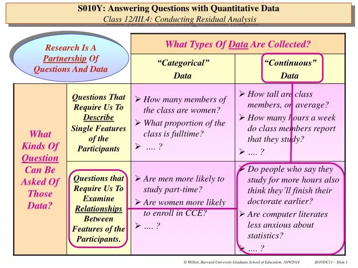
What Types Of Data Are Collected?. Research Is A Partnership Of Questions And Data. “Categorical” Data. “Continuous” Data. S010Y: Answering Questions with Quantitative Data Class 12/III.4: Conducting Residual Analysis. What Kinds Of Question Can Be Asked Of Those Data?.

E N D
What Types Of Data Are Collected? Research Is A Partnership Of Questions And Data “Categorical” Data “Continuous” Data S010Y: Answering Questions with Quantitative DataClass 12/III.4: Conducting Residual Analysis What Kinds Of Question Can Be Asked Of Those Data? Questions That Require Us To Describe Single Features of the Participants • How many members of the class are women? • What proportion of the class is fulltime? • …. ? • How tall are class members, on average? • How many hours a week do class members report that they study? • …. ? Questions that Require Us To Examine Relationships Between Features of the Participants. • Are men more likely to study part-time? • Are women more likely to enroll in CCE? • …. ? • Do people who say they study for more hours also think they’ll finish their doctorate earlier? • Are computer literates less anxious about statistics? • …. ?
Here are the PC-SAS data input statements that you’ve come to know and love Here’s the OLS regression analysis, using PROC REG, that you’ve seen before (with one additional line that we will discuss later). Standard scatterplot of the HSGRADRT vs. STRATIO relationship Having examined the “smooth” with regression analysis, let’s examine the “rough” with residual analysis … OPTIONS Nodate Pageno=1; TITLE1 'A010Y: Answering Questions with Quantitative Data'; TITLE2 'Class 11/Handout 1: Dissecting Relationships Between Continuous Variables'; TITLE3 'The Infamous Wallchart Data'; TITLE4 'Data in WALLCHT.txt'; *--------------------------------------------------------------------------------* Input data, name and label variables in the dataset *--------------------------------------------------------------------------------*; DATA WALLCHT; INFILE 'C:\DATA\A010Y\WALLCHT.txt'; INPUT STATE $ TCHRSAL STRATIO PPEXPEND HSGRADRT; LABEL TCHRSAL = '1988 Average Teacher Salary' STRATIO = '1988 Student/Teacher Ratio' PPEXPEND = '1988 Expenditure/Student' HSGRADRT = '1988 Statewide H.S. Graduation Rate'; *--------------------------------------------------------------------------------* Representing the nature of the relationship of HSGRADRT and STRATIO *--------------------------------------------------------------------------------*; PROC REG DATA=WALLCHT; TITLE5 'OLS Regression of H.S. Graduation Rate on Student/Teacher Ratio'; MODEL HSGRADRT = STRATIO; OUTPUT OUT=DIAGNOSE R=RAWRESID P=PREDVAL; PROC PLOT DATA=WALLCHT; TITLE5 'Plot of H.S. Graduation Rates against Student/Teacher Ratios'; PLOT HSGRADRT*STRATIO / HAXIS = 10 TO 25 BY 5 VAXIS = 50 TO 100 BY 10; S010Y: Answering Questions with Quantitative Data Class 12/III.4: Conducting Residual Analysis
These “Parameter Estimates” provide the fitted trend line as the following fitted model: Slope Intercept Here’s the regression output that you’ve seen before, and which specifies the fitted regression line….. Dependent Variable: HSGRADRT 1988 Statewide H.S. Graduation Rate Parameter Estimates Parameter Standard Variable Label DF Estimate Error t Value Intercept Intercept 1 93.69187 7.95093 11.78 STRATIO 1988 Student/Teacher Ratio 1 -1.12140 0.45516 -2.46 Parameter Estimates Variable Label DF Pr > |t| Intercept Intercept 1 <.0001 STRATIO 1988 Student/Teacher Ratio 1 0.0174 S010Y: Answering Questions with Quantitative Data Class 12/III.4: Conducting Residual Analysis
The fitted equation is telling us PROC REG’s best prediction for HSGRADRT at every value of STRATIO. For instance… 1. When STRATIO = 13.3 (the minimum value of STRATIO), Predicted value of HSGRADRT = (93.69) + (-1.12)(13.3) = 93.69 – 14.90 = 78.8 Plot these values to obtain the fitted trend line 2. When STRATIO = 24.7 (the maximum value of STRATIO), Predicted value of HSGRADRT = (93.69) + (-1.12)(24.7) = 93.69 – 27.66 = 66.0 Here’s the fitted regression model that you recognize … S010Y: Answering Questions with Quantitative Data Class 12/III.4: Conducting Residual Analysis
78.8 66.0 13.3 24.7 This provides us with the “smooth” – where’s the “rough”? … 1 100 ˆ 9 ‚ 8 ‚ 8 ‚ ‚ S ‚ t ‚ A a 90 ˆ t ‚ A A e ‚ A w ‚ A A i ‚ A A d ‚ e ‚ 80 ˆ B A A H ‚ A A . ‚ A A A A S ‚ A A A A . ‚ A A AA A A A A ‚ A G ‚ AA A A r 70 ˆ A A a ‚ A A d ‚ A A u ‚ B A a ‚ A t ‚ A i ‚ AB o 60 ˆ n ‚ A ‚ R ‚ a ‚ t ‚ e ‚ 50 ˆ Šƒƒˆƒƒƒƒƒƒƒƒƒƒƒƒƒƒƒƒƒƒƒƒƒˆƒƒƒƒƒƒƒƒƒƒƒƒƒƒƒƒƒƒƒƒƒˆƒƒƒƒƒƒƒƒƒƒƒƒƒƒƒƒƒƒƒƒƒˆƒƒ 10 15 20 25 1988 Student/Teacher Ratio Now, to examine the rough … Let’s pick a few states, and compare our predictions of HS graduation rate to the actual observedvalues. We call this the “analysis of residuals”… S010Y: Answering Questions with Quantitative Data Class 12/III.4: Conducting Residual Analysis
90.9 74.4 17.1 Here’s the “rough” for Minnesota … • How about Minnesota? • Observed valuesof the outcome and the predictor: • STRATIO = 17.1 • HSGRADRT = 90.9, & • Predicted valueof HSGRADRT, obtained from fitted regression line: 1 100 ˆ 9 ‚ 8 ‚ 8 ‚ ‚ S ‚ t ‚ A a 90 ˆ t ‚ A A e ‚ A w ‚ A A i ‚ A A d ‚ e ‚ 80 ˆ B A A H ‚ A A . ‚ A AAA S ‚ A AAA . ‚ A A AA A AAA ‚ A G ‚ AA A A r 70 ˆ A A a ‚ A A d ‚ A A u ‚ B A a ‚ A t ‚ A i ‚ AB o 60 ˆ n ‚ A ‚ R ‚ a ‚ t ‚ e ‚ 50 ˆ Šƒƒˆƒƒƒƒƒƒƒƒƒƒƒƒƒƒƒƒƒƒƒƒƒˆƒƒƒƒƒƒƒƒƒƒƒƒƒƒƒƒƒƒƒƒƒˆƒƒƒƒƒƒƒƒƒƒƒƒƒƒƒƒƒƒƒƒƒˆƒƒ 10 15 20 25 1988 Student/Teacher Ratio S010Y: Answering Questions with Quantitative Data Class 12/III.4: Conducting Residual Analysis
69.5 69.1 Here’s the “rough” for Hawaii … • How about Hawaii? • Observed values of the outcome and the predictor: • HSGRADRT = 69.1, & • STRATIO = 21.6 • Predicted value of HSGRADRT: 1 100 ˆ 9 ‚ 8 ‚ 8 ‚ ‚ S ‚ t ‚ A a 90 ˆ t ‚ A A e ‚ A w ‚ A A i ‚ A A d ‚ e ‚ 80 ˆ B A A H ‚ A A . ‚ A A A A S ‚ A A A A . ‚ A A AA A A A A ‚ A G ‚ AA A A r 70 ˆ A A a ‚ A A d ‚ A A u ‚ B A a ‚ A t ‚ A i ‚ AB o 60 ˆ n ‚ A ‚ R ‚ a ‚ t ‚ e ‚ 50 ˆ Šƒƒˆƒƒƒƒƒƒƒƒƒƒƒƒƒƒƒƒƒƒƒƒƒˆƒƒƒƒƒƒƒƒƒƒƒƒƒƒƒƒƒƒƒƒƒˆƒƒƒƒƒƒƒƒƒƒƒƒƒƒƒƒƒƒƒƒƒˆƒƒ 10 15 20 25 1988 Student/Teacher Ratio S010Y: Answering Questions with Quantitative Data Class 12/III.4: Conducting Residual Analysis 21.6
76.7 Here’s the “rough” for Minnesota … • How about New York State? • Observed values of the outcome and the predictor: • HSGRADRT = 62.3, & • STRATIO = 15.2 • Predicted value of HSGRADRT: 1 100 ˆ 9 ‚ 8 ‚ 8 ‚ ‚ S ‚ t ‚ A a 90 ˆ t ‚ A A e ‚ A w ‚ A A i ‚ A A d ‚ e ‚ 80 ˆ B A A H ‚ A A . ‚ A A A A S ‚ A A A A . ‚ A A AA A A A A ‚ A G ‚ AA A A r 70 ˆ A A a ‚ A A d ‚ A A u ‚ B A a ‚ A t ‚ A i ‚ AB o 60 ˆ n ‚ A ‚ R ‚ a ‚ t ‚ e ‚ 50 ˆ Šƒƒˆƒƒƒƒƒƒƒƒƒƒƒƒƒƒƒƒƒƒƒƒƒˆƒƒƒƒƒƒƒƒƒƒƒƒƒƒƒƒƒƒƒƒƒˆƒƒƒƒƒƒƒƒƒƒƒƒƒƒƒƒƒƒƒƒƒˆƒƒ 10 15 20 25 1988 Student/Teacher Ratio S010Y: Answering Questions with Quantitative Data Class 12/III.4: Conducting Residual Analysis 62.3 15.2
On a scatterplot with a fitted regression line, the “vertical distance” between the observed value of HSGRADRTand its predicted valueis called the residual….. S010Y: Answering Questions with Quantitative Data Class 12/III.4: Conducting Residual Analysis • Residuals can be informative and useful: • Residuals represent individual deviations from the average trend: • They tell us about HSGRADRT, while taking “into account” or “controlling for” STRATIO. • They tell us whether states are doing “better” or “worse” than we would have predicted, given our knowledge of their student/teacher ratio.
You can ask PC-SAS to compute the residuals for you, and to output them into a diagnostic dataset, for you to explore. P = PREDVAL P command tells PC-SAS that you also want to put the predicted values into the new output dataset, and call them PREDVAL. OUT = DIAGNOSE OUT command tells PC-SAS that you want to create an OUTput dataset called DIAGNOSE. R = RAWRESID R command tells PC-SAS that you want to put “raw residuals” into the new output dataset, and call them RAWRESID We don’t have to compute the residuals and predictedvalues by hand…. <titling and input lines omitted>> *------------------------------------------------------------------------* Representing the nature of the relationship of HSGRADRT and STRATIO *------------------------------------------------------------------------*; PROC REG DATA=WALLCHT; TITLE5 'OLS Regression of H.S. Graduation Rate on Student/Teacher Ratio'; MODEL HSGRADRT = STRATIO; OUTPUT OUT=DIAGNOSE R=RAWRESID P=PREDVAL; S010Y: Answering Questions with Quantitative DataClass 12/III.4: Conducting Residual Analysis
You can use PROCUNIVARIATE to explore the sample distribution of the raw residuals across the states. You can use PROCPLOT to plot the raw residuals against the predictor. You can use PROC SORT to sort the states by the value of their raw residual, and then use PROCPRINT to list them all out for inspection, along with the name of the state, and the observed and predicted values of HSGRADRT Once the residuals and predictedvalues are output to the DIAGNOSE dataset, you can take a look…. *-------------------------------------------------------------------------------* Examining the distribution of the raw residuals *-------------------------------------------------------------------------------*; PROC UNIVARIATE PLOT DATA=DIAGNOSE; TITLE5 'Univariate descriptive statistics on the Raw Residuals'; VAR RAWRESID; ID STATE; PROC PLOT DATA=DIAGNOSE; TITLE5 'Plot of the Raw Residuals against the Values of the Predictor, STRATIO'; PLOT RAWRESID*STRATIO / HAXIS = 10 TO 25 BY 10 VREF = 0; *-------------------------------------------------------------------------------* Reranking the States based on the value of their raw residuals *-------------------------------------------------------------------------------*; PROC SORT DATA=DIAGNOSE; BY DESCENDING RAWRESID; PROC PRINT LABEL DATA=DIAGNOSE; TITLE5 'Listing of State Observed, Predicted and Residual Graduation Rates'; VAR STATE HSGRADRT PREDVAL RAWRESID; S010Y: Answering Questions with Quantitative Data Class 12/III.4: Conducting Residual Analysis
Sample mean of the raw residuals is exactly zero! Sample standard deviation of the raw residuals is 7.4 . This number can be quite useful! Listing of “extreme observations” is useful for identifying states whose observed values of HSGRADRT are wildly different from their predicted values Here are some of the univariate descriptive statistics on the residuals…. Variable: RAWRESID (Residual) N 50 Sum Weights 50 Mean 0 Sum Observations 0 Std Deviation 7.38040638 Variance 54.4703983 Basic Statistical Measures Location Variability Mean 0.00000 Std Deviation 7.38041 Median -0.27000 Variance 54.47040 Mode . Range 32.56358 Interquartile Range 8.69773 Quantile Estimate 100% Max 16.384021 95% 12.101925 75% Q3 4.760352 50% Median -0.269997 25% Q1 -3.937376 5% -11.733883 0% Min -16.179560 Extreme Observations -----------Lowest----------- -----------Highest---------- Value STATE Obs Value STATE Obs -16.1796 FL 9 10.8684 WY 50 -14.3466 NY 32 11.3262 MT 26 -11.7339 AZ 3 12.1019 ND 34 -11.7217 GA 10 13.4066 UT 44 -11.5460 LA 18 16.3840 MN 23 S010Y: Answering Questions with Quantitative Data Class 12/III.4: Conducting Residual Analysis
Actually, for the p-values that were computed in the regression analysis to be correct, the residuals must be normally distributed: • You can use stem.leafand box plotsto check roughly if this assumption holds in your analysis. Here’s the stem.leaf and boxplot of the residual… Stem Leaf # Boxplot 16 4 1 | 14 | 12 14 2 | 10 93 2 | 8 646 3 | 6 111 3 | 4 89 2 +-----+ 2 2779938 7 | | 0 6722 4 | + | -0 6566442 7 *-----* -2 9870641 7 +-----+ -4 73 2 | -6 16 2 | -8 808 3 | -10 775 3 | -12 | -14 3 1 | -16 2 1 | ----+----+----+-- S010Y: Answering Questions with Quantitative Data Class 12/III.4: Conducting Residual Analysis
+2 sd +1 sd -1 sd -2 sd H.S. Predicted Graduation Value of STATE Rate HSGRADRT Residual MN 90.9 74.5160 16.3840 UT 79.4 65.9934 13.4066 ND 88.3 76.1981 12.1019 MT 87.3 75.9738 11.3262 WY 88.3 77.4316 10.8684 IA 85.8 76.1981 9.6019 WI 84.9 75.5252 9.3748 NE 85.4 76.7588 8.6412 CT 84.9 78.7773 6.1227 OH 79.6 73.5067 6.0933 WA 77.1 71.0396 6.0604 ID 75.4 70.4789 4.9211 NV 75.8 71.0396 4.7604 KS 80.2 76.4224 3.7776 SD 79.6 76.3102 3.2898 PE 78.4 75.5252 2.8748 AL 74.9 72.0489 2.8511 AR 77.2 74.5160 2.6840 IN 76.3 73.6189 2.6811 MI 73.6 71.3761 2.2239 IL 75.6 74.4038 1.1962 CO 74.7 73.5067 1.1933 WV 77.3 76.6466 0.6534 VT 78.7 78.1044 0.5956 Here are the individual states, ordered by their residuals … S010Y: Answering Questions with Quantitative Data Class 12/III.4: Conducting Residual Analysis OR 73.0 73.1703 -0.1703 HI 69.1 69.4697 -0.3697 MD 74.1 74.5160 -0.4160 NJ 77.4 77.9923 -0.5923 NM 71.9 72.4975 -0.5975 MO 74.0 75.5252 -1.5252 NH 74.1 75.7495 -1.6495 CA 65.9 68.0119 -2.1119 TN 69.3 71.7125 -2.4125 ME 74.4 76.9831 -2.5831 OK 71.7 74.7403 -3.0403 MA 74.4 78.1044 -3.7044 VA 71.6 75.4131 -3.8131 DL 71.7 75.6374 -3.9374 KY 69.0 73.2824 -4.2824 MS 66.9 72.6096 -5.7096 NC 66.7 73.2824 -6.5824 RI 69.8 76.8709 -7.0709 AK 65.5 74.2917 -8.7917 TX 65.3 74.2917 -8.9917 SC 64.6 74.4038 -9.8038 LA 61.4 72.9460 -11.5460 GA 61.0 72.7217 -11.7217 AZ 61.1 72.8339 -11.7339 NY 62.3 76.6466 -14.3466 FL 58.0 74.1796 -16.1796 • Which are the truly extraordinary states? • If the residuals are normally distributed, then the truly extraordinary states may be those that lie ±2 standard deviations (= ± 2×7.4) from the mean? • The mean of the residuals is zero.
1 100 ˆ 9 ‚ 8 ‚ 8 ‚ ‚ S ‚ t ‚ A a 90 ˆ t ‚ A A e ‚ A w ‚ A A i ‚ A A d ‚ e ‚ 80 ˆ B A A H ‚ A A . ‚ A A A A S ‚ A A A A . ‚ A A AA A A A A ‚ A G ‚ AA A A r 70 ˆ A A a ‚ A A d ‚ A A u ‚ B A a ‚ A t ‚ A i ‚ AB o 60 ˆ n ‚ A ‚ R ‚ a ‚ t ‚ e ‚ 50 ˆ Šƒƒˆƒƒƒƒƒƒƒƒƒƒƒƒƒƒƒƒƒƒƒƒƒˆƒƒƒƒƒƒƒƒƒƒƒƒƒƒƒƒƒƒƒƒƒˆƒƒƒƒƒƒƒƒƒƒƒƒƒƒƒƒƒƒƒƒƒˆƒƒ 10 15 20 25 1988 Student/Teacher Ratio An Enhanced Conclusion… In our investigation of state-level aggregate statistics, the average percentage of seniors graduating from High School is related to the average student/teacher ratio in the state. With state-wide high-school graduation rate (HSGRADRT) as outcome and state-wide student/teacher ratio (STRATIO) as predictor, the trend-line estimated by OLS regression analysis has a slope of –1.12 (p = 0.0174). This suggests that two states whose student/teacher ratios differ by 1 student per teacher will tend to have graduation rates that differ by 1.12 percentage points, where states that enjoy lower student/teacher ratios having higher high-school graduation rates … <<substantive conjecture follows …>> However, not all states follow the average trend. Some states graduate high-school seniors at rates considerably different from those predicted from knowledge of their student/teacher ratios. In particular, Minnesota has a very large positive residual indicating that its high-school graduation rate is much higher than we would expect, based on its student/teacher ratio. Florida, on the other hand, has a very large negative residual indicating that it is graduating high-school seniors at a rate that is much lower than we would anticipate … <<substantive conjecture follows …>> S010Y: Answering Questions with Quantitative Data Class 12/III.4: Conducting Residual Analysis