Download
1 / 19
190 likes | 309 Views
Intercomparison of tropospheric ozone measurements from TES and OMI. Lin Zhang 1 , Daniel J. Jacob 1 , Xiong Liu 2,3 , Jennifer A. Logan 1 , and the TES Science Team. 1. Harvard University 2. GEST, UMBC 3. Harvard-Smithsonian Center for Astrophysics. TES Science Team Meeting (Feb.24, 2009).

E N D
Intercomparison of tropospheric ozone measurements from TES and OMI Lin Zhang1, Daniel J. Jacob1, Xiong Liu2,3, Jennifer A. Logan1, and the TES Science Team 1. Harvard University 2. GEST, UMBC 3. Harvard-Smithsonian Center for Astrophysics TES Science Team Meeting (Feb.24, 2009)
Concurrent ozone measurements from IR and UV • OMI • Nadir-looking instrument measuring backscattered solar radiation (270-500 nm) • Daily global coverage at a spatial resolution of 13 x 24 km2 at nadir • Retrieve ozone at 24 ~2.5 km layers • TES • Infrared-imaging Fourier transform spectrometer (3.3-15.4 µm) • 16 orbits of nadir vertical profiles at a spatial resolution of 5x8 km2 and spaced 1.6° along the orbit track every other day. • Retrievals of ozone and CO at 67 levels from surface up to 0.1 hPa, version 3 data Do they provide consistent measurements of tropospheric ozone? What can we learn by comparing both measurements with chemical transport models?
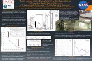
Vertical sensitivity of TES and OMI ozone retrievals Both retrievals are obtained from the optimal estimation method [Rodgers, 2000]: Retrieval Averaging kernel Aug 6, 2009 58W, 28N 1.8 DOFS in the troposphere 1.0 DOFS in the troposphere
Tropospheric ozone from TES and OMI 2006 ozone at 500 hPa averaged on 4ox5o resolution OMI observations are selected along TES pixels. The data are reprocessed with a single fixed a priori.
Tropospheric ozone from TES, OMI and GEOS-Chem 2006 ozone at 500 hPa averaged on 4ox5o resolution The data and model results are reprocessed with a single fixed a priori. GEOS-Chem simulation in 4ox5o resolution is sampled along the TES/OMI pixels, and then smoothed by corresponding averaging kernels.
Validation with ozonesonde Ozonesonde data from 2005-2007, available at AURA AVDC Coincidence Criteria: < 2o longitudes & Latitudes, < 10 hours 60oS-60oN, 500 hPa: TES has a positive bias of 5.4 ± 9 ppbv OMI has a positive bias of 3.1± 5 ppbv
Methods for the intercomparison Sparse in time and space Validation Validation 1. Sonde method: Validation with ozonesonde measurements
Methods for the intercomparison Sparse in time and space Validation Validation Direct comparison (Rodgers and Conner, 2003) 1. Sonde method: Validation with ozonesonde measurements 2. Direct method: Compare OMI/TES directly after considering their different a priori constrains and vertical sensitivity (Apply OMI averaging kernels to TES retrievals)
Methods for the intercomparison Sparse in time and space Validation Validation Evaluation Interpretation Evaluation Evaluation Interpretation Interpretation Direct comparison (Rodgers and Conner, 2003) 1. Sonde method: Validation with ozonesonde measurements 2. Direct method: Compare OMI/TES directly after considering their different a priori constrains and vertical sensitivity (Apply OMI averaging kernels to TES retrievals) 3. CTM method: Use GEOS-Chem CTM as a comparison platform
What do the methods actually compare? Let • Sonde method:TES – sonde/TES AK = bTES • OMI – sonde/OMI AK = bOMI • TES – OMI = bTES–bOMI 2. Direct method: AOMIbTES – bOMI + AOMI(ATES – I)(X – Xa) (Rodgers and Conner, 2003) 3. CTM method: (TES – CTM/TES AK) – (OMI – CTM/OMI AK) = bTES – bOMI + (ATES – AOMI)(X – XCTM)
Quantify differences between TES and OMI 1. TES – OMI (sonde) = bTES – bOMI 2. TES (OMI AK) – OMI = AOMIbTES – bOMI + AOMI(ATES – I)(X – Xa) 3. TES – OMI (GC) = bTES – bOMI + (ATES – AOMI)(X – XCTM) 500 hPa 160 TES/OMI/sonde coincidences for 2006 CTM method Direct method In the direct method, slopes < 1 reflect application of AOMI reduce the sensitivity to diagnose the bias. The CTM method preserves the variability of the differences in the comparison. TES – OMI Sonde method [ppbv] 850 hPa CTM method Direct method TES – OMI Sonde method [ppbv]
Difference between TES and OMI at 500 hPa TES – OMI Direct method Sonde method CTM method 2.6 ± 6.6 ppbv -0.1 ± 3.6 ppbv -0.3 ± 5.0 ppbv TES – OMI Mean ± 1 sigma Total error for both TES and OMI
Difference between TES and OMI at 850 hPa TES – OMI Direct method Sonde method CTM method 3.3 ± 6.8 ppbv -0.3 ± 1.9 ppbv 2.7 ± 5.5 ppbv TES – OMI Mean ± 1 sigma
Differences with GEOS-Chem at 500 hPa For 2006 and averaged on 4ox5o resolution Minus 3 ppbv from both TES and OMI measurements. Regions with the bias between TES and OMI larger than 10 ppbv are masked as black. GC – sonde GC/TES AK – (TES– 3) GC/OMI AK – (OMI– 3)
Differences with GEOS-Chem at 500 hPa For 2006 and averaged on 4ox5o resolution Minus 3 ppbv from both TES and OMI measurements. Regions with the bias between TES and OMI larger than 10 ppbv are masked as black. GC – sonde GC/TES AK – (TES– 3) GC/OMI AK – (OMI– 3)
Tropospheric ozone measurements from TES and OMI 2006 ozone at 500 hPa averaged on 4ox5o resolution OMI observations are sampled along the TES pixels. Convert the different a priori to a fixed a priori:
Vertical sensitivity of TES and OMI ozone retrievals Both retrievals are obtained from the optimal estimation method [Rodgers, 2000]: Averaging kernel OMI Degrees of Freedom for tropospheric ozone July 2006 TES Zonal average of Diagonal terms of AK