Download
1 / 11
110 likes | 277 Views
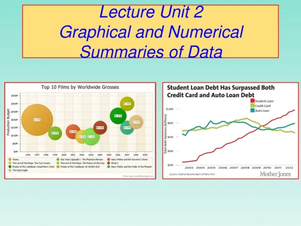
Chapter 2 Exploring Data with Graphs and Numerical Summaries. Section 2.3 Measuring the Center of Quantitative Data. The mean is the sum of the observations divided by the number of observations. Mean. Example: Center of the Cereal Sodium Data.

E N D
Chapter 2Exploring Data with Graphs and Numerical Summaries Section 2.3 Measuring the Center of Quantitative Data
The mean is the sum of the observations divided by the number of observations. Mean
Example: Center of the Cereal Sodium Data We find the mean by adding all the observations and then dividing this sum by the number of observations, which is 20: 0, 340, 70, 140, 200, 180, 210, 150, 100, 130, 140, 180, 190, 160, 290, 50, 220, 180, 200, 210 Mean = (0 + 340 + 70 + . . . +210)/20 = 3340/20 =167
The median is the midpoint of the observations when they are ordered from the smallest to the largest (or from the largest to smallest). How to Determine the Median: Put the n observations in order of their size. If the number of observations, n, is: odd, then the median is the middle observation. even, then the median is the average of the two middle observations. Median
CO2 pollution levels in 8 largest nations measured in metric tons per person: China 4.9 Brazil 1.9 India 1.4 Pakistan 0.9 United States 18.9 Russia 10.8 Indonesia 1.8 Bangladesh 0.3 The CO2 values have n = 8 observations. The ordered values are: 0.3, 0.9, 1.4, 1.8, 1.9, 4.9, 10.8, 18.9 Example: CO2 Pollution
Since n is even, two observations are in the middle, the fourth and fifth ones in the ordered sample. These are 1.8 and 1.9. The median is their average, 1.85. The relatively high value of 18.9 falls well above the rest of the data. It is an outlier. The size of the outlier affects the calculation of the mean but not the median. Example: CO2 Pollution
The shape of a distribution influences whether the mean is larger or smaller than the median. Perfectly symmetric, the mean equals the median. Skewed to the right, the mean is larger than the median. Skewed to the left, the mean is smaller than the median. Comparing the Mean and Median
In a skewed distribution, the mean is farther out in the long tail than is the median. For skewed distributions the median is preferred because it is better representative of a typical observation. Comparing the Mean and Median Figure 2.9 Relationship Between the Mean and Median. Question: For skewed distributions, what causes the mean and median to differ?
A numerical summary measure is resistant if extreme observations (outliers) have little, if any, influence on its value. The Medianis resistant to outliers. The Meanis not resistant to outliers. Resistant Measures
Mode Value that occurs most often. Highest bar in the histogram. The mode is most often used with categorical data. The Mode