Download
1 / 27
400 likes | 930 Views
Solving Ordinary Differential Equations. Application of Unsteady Flow form an Orifice. Ordinary Differential Equations. General Form:. for sake of simplicity only consider linear case:. Finite Difference Methods. Approx. sol’n. Exact sol’n.

E N D
Solving Ordinary Differential Equations Application of Unsteady Flow form an Orifice
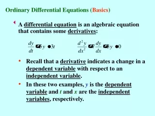
Ordinary Differential Equations General Form: for sake of simplicity only consider linear case:
Finite Difference Methods Approx. sol’n Exact sol’n Third - Approximate using the discrete Basic Concepts First - Discretize Time Second - Represent x(t) using values at ti
Finite Difference Methods Forward Euler Approximation (Explicit method)
1 γH2O 2 Z = 0 A2 3 Example: FDM Forward Euler • Phenomenon: Flow through Orifice at Variable Head h
Choice of Time Step • The choice of time step is based on the idea that the values do not change too much during the time step. • Change of 5% in the initial value of the head h during the first time step is acceptable from engineering point of view. This is your judgment as a modeller.
Numerical Example • Initial head h(t=0)= 5 m, cd=0.95, do=0.1 m, D=5 m. • Calculate the falling of the water level in time until the tank is empty. Draw h(t) over t. • Check your results with analytical solution.
Estimation of time step • 5% of h(0)= 0.05*5=0.25 m • H(n+1)=5-0.25=4.75 m
Modified Euler (Predictor-Corrector) Method • Also “explicit” • next h is an explicit function of previous • But evaluate h at a some times to get a better estimate of next h • E.g. midpoint method:
Finite Difference Methods Backward Euler Approximation (Implicit method)
Finite Difference Methods Backward Euler Algorithm Solve with Gaussian Elimination
Finite Difference Methods Trapezoidal Rule Algorithm Solve with Gaussian Elimination
Finite Difference Methods Numerical Integration View Trap BE FE
Finite Difference Methods Summary of Basic Concepts Trap Rule, Forward-Euler, Backward-Euler Are all one-step methods Forward-Euler is simplest No equation solution explicit method. Boxcar approximation to integral Backward-Euler is more expensive Equation solution each step implicit method Trapezoidal Rule might be more accurate Equation solution each step implicit method Trapezoidal approximation to integral