Download
1 / 53
530 likes | 591 Views
Learn how to create subplots and 3D graphics, control GUI properties, and make decisions in the "Game of Life" simulation. Discover essential Matlab commands for interacting with figures and axes, setting properties, and creating visualizations using surf, meshgrid, colormap, shading, and view functions.

E N D
More Matlab Graphics and GUI Graphics subplots some useful commands 3D graphics GUI GUI controls The callback property Other essential properties
Comments about the “Game of Life” Initial universe Time step
Time step input universe embed Count neighbors Make decisions output universe
Count neighbors input universe Count the neighbors of a cell Matrix with the neighbors numbers
Subplot II Subplots Subplot I
h1 = subplot(7,7,[1 2 3 4 5 6 ... 8 9 10 11 12 13 ... 15 16 17 18 19 20 ... 22 23 24 25 26 27 ... 29 30 31 32 33 34 ... 36 37 38 19 40 41]);
h1 = subplot(7,7,[1 2 3 4 5 6 ... 8 9 10 11 12 13 ... 15 16 17 18 19 20 ... 22 23 24 25 26 27 ... 29 30 31 32 33 34 ... 36 37 38 19 40 41]); get(h1,'type') ans = axes
h1 = subplot(7,7,[1 2 3 4 5 6 ... 8 9 10 11 12 13 ... 15 16 17 18 19 20 ... 22 23 24 25 26 27 ... 29 30 31 32 33 34 ... 36 37 38 19 40 41]); subplot(7,7,[7 14])
Useful Commands The interactively edited figure/axes/object is accessible through the gcf/gca/gcocommands (get current figure/axes/object). >> get(gca) ALim = [0 1] ALimMode = auto AmbientLightColor = [1 1 1] Box = on CameraPosition = [5.5 5.5 17.3205] CameraPositionMode = auto CameraTarget = [5.5 5.5 0] CameraTargetMode = auto CameraUpVector = [0 1 0] CameraUpVectorMode = auto CameraViewAngle = [6.60861] CameraViewAngleMode = auto :
hl=findobj(gcf,’type’,’line’) set(h1,'color','r');
set(gcf,'tag','first‘); Figure; y = x.^-2; plot(x,y);
firstFigure = findobj('tag','first'); h2 = findobj(firstFigure,'type','line') set(h2,'marker','*');
firstFigure = findobj('tag','first'); h2 = findobj(firstFigure,'type','line') set(h2,'marker','*');
We want to calculate and display Z=x(x2-y2) 3D graphics x = [-2:0.2:2] x = [ -2 -1.8 …. 1.8 2] y = [-4:0.4:4] y = [ -4 -3.6 …. 3.6 4]
length(y) rows replica of x 3D graphics surf(XX,YY,ZZ) size(XX) ans = 21 21 XX(1:5,1:5) ans = -2.0000 -1.8000 -1.6000 -1.4000 -1.2000 …. -2.0000 -1.8000 -1.6000 -1.4000 -1.2000 …. -2.0000 -1.8000 -1.6000 -1.4000 -1.2000 …. -2.0000 -1.8000 -1.6000 -1.4000 -1.2000 …. -2.0000 -1.8000 -1.6000 -1.4000 -1.2000 …. . .
surf(XX,YY,ZZ) size(XX) ans = 21 21 XX(1:5,1:5) ans = -2.0000 -1.8000 -1.6000 -1.4000 -1.2000 …. -2.0000 -1.8000 -1.6000 -1.4000 -1.2000 …. -2.0000 -1.8000 -1.6000 -1.4000 -1.2000 …. -2.0000 -1.8000 -1.6000 -1.4000 -1.2000 …. -2.0000 -1.8000 -1.6000 -1.4000 -1.2000 …. . .
surf(XX,YY,ZZ) size(XX) ans = 21 21 XX(1:5,1:5) ans = -2.0000 -1.8000 -1.6000 -1.4000 -1.2000 …. -2.0000 -1.8000 -1.6000 -1.4000 -1.2000 …. -2.0000 -1.8000 -1.6000 -1.4000 -1.2000 …. -2.0000 -1.8000 -1.6000 -1.4000 -1.2000 …. -2.0000 -1.8000 -1.6000 -1.4000 -1.2000 …. . .
Length(x) columns replica of y 3D graphics surf(XX,YY,ZZ) size(YY) ans = 21 21 YY(1:5,1:5) ans = -4.0000 -4.0000 -4.0000 -4.0000 -4.0000 …. -3.6000 -3.6000 -3.6000 -3.6000 -3.6000 …. -3.2000 -3.2000 -3.2000 -3.2000 -3.2000 …. -2.8000 -2.8000 -2.8000 -2.8000 -2.8000 …. -2.4000 -2.4000 -2.4000 -2.4000 -2.4000 …. . .
Element-by-element matrix operations 3D graphics surf(XX,YY,ZZ) size(ZZ) ans = 21 21 ZZ = XX.*(XX.^2-YY.^2);
How do we create XX and YY? [XX YY] = meshgrid(x,y); Were [XX YY] = meshgrid(x) is the same as [XX YY] = meshgrid(x,x);
How does Matlab know how to relate some value with a specific color? • Colormaps! • A colormap is an m-rows by 3 column matrix • Each row is a color specified in RGB values(between 0 and 1) C=get(1,'colormap') C = 00 0.5625 00 0.6250 ... ... ... 0.5625 1.0000 0.4375 0.6250 1.0000 0.3750 ... ... ... 0.6250 00 0.5625 00 0.5000 00
“colormap” is a property of the figure colormap(cool)
The same plot as a contour map colormap(jet) contour(XX,YY,ZZ,100)
… and with a colorbar colorbar
flat faceted flat faceted %default interp >>shading interpolated Solid shading • We can change the way the surface displays by changing its shading: >>surf(peaks) %creates 49 by 49 matrix % an plots its values %against x,y indices
Every axes has a property called ‘view’ that controls the azimuth (az) and elevation (el) of the viewpoint • To change the viewpoint we use either: • view(az,el) or • set(axes_handle,’View’,[az el])
>>view(-37.5,30) >>view(-10.0,30) >>view(0,0) >>view(0,30)
Special 3d plots • contour3(x,y,z,n) %create n realistic contours interpreting z • %as the height from the x y plane. If specified • % x and y should have the same size as z • >>contour3(topo,30) • >>axis off
Special 3d plots • We can create a sphere or a cylinder (of radius =1) with little effort • >>[x,y,z]=sphere; %will compute the required % N+1 (N=20 by default) coordinates so • >>surf(x,y,z) %will plot sphere surface • >>axis equal • Note: • sphere without left arguments will plot the surface. • sphere(n) use n instead of the default of 20
Special 3d plots • To create a cylinder we issue the following command: • >>[x,y,z]=cylinder; • >>surf(x,y,z)%this creates a basic cylinder of %radius 1
Special 3d plots • We can also create cylinder with reference to a specific profile. We will now generate a cylinder with the esin(t) profile >> t = 0:pi/10:2*pi; >> [X,Y,Z] = cylinder(exp(sin(t))); >> surf(X,Y,Z)
Graphical User Interfaces • Why? • Built in UIs • Uicontrols • GUI programming
Graphic Objects • figure • axes • 2D-plot • 3D-plot • axis labels • title • GUI objects • pushbutton • toggle • edit • text • menu
Motivation or why GUIs? • Enable you to share your work with other people (your advisor/lab mates or grandmother) • Easy way to perform repetitive task that need constant user input • Create interactive demos to your applications • It’s fun…
GUI components • Figure window • GUI controllers which are divided into two major classes: • uimenu (like the File,Edit etc) • uicontrols (buttons, lists, radio buttons pop-up list like in any other application) • uimenu and uicontrols are children of the figure • If an uimenu is implemented as submenu, then it is a child of another uimenu
Interface controllers • The UIcontrols are common interface controlers • Help us perform specific actions or set the variables for future actions • Actions and options are selected by the mouse, some UIcontrols are also editable so we can use the keyboard as well
Interface controllers • We can create UIcontrols simply by implementing the following syntax • handle_to_UI=uicontrol(‘Property Name’,’Property Value’);
Interface controllers • UIcontrol types are defined by their ‘style’ property:
Interface controllersare graphic objects • Essential properties: • Callback – A string with one or more commands that is executed when the controller is activated. • May be empty – ''