Download
1 / 64
680 likes | 938 Views
Planarity Testing And Embedding. By: Seyed Akbar Mostafavi Fall 2010. Outline. Planar Graphs Planarity Testing Theorems Kuratowski’s Theorem Demoucron’s Planarity Algorithms Euler Polyhedron Formula Nonplanarity of Kuratowski Graphs Minimum Degree Bound

E N D
Planarity Testing And Embedding By: Seyed Akbar Mostafavi Fall 2010
Outline • Planar Graphs • Planarity Testing Theorems • Kuratowski’s Theorem • Demoucron’s Planarity Algorithms • Euler Polyhedron Formula • Nonplanarity of Kuratowski Graphs • Minimum Degree Bound • Definitions of Planarity Testing • st-numbering Algorithm • Bush Form and PQ-Tree • Booth-Lueker Algorithm • Embedding Algorithms
Planar Graphs • A graph G(V,E) is called planar graph if it can be drawn on embedded in the plane in such a way that the edges of the embedding intersect only at the vertices of G. • Example: K(4)
Planar Graphs • Nonplanar Graph example: K(3,3)
Planarity Testing • Two classical approaches • Theorem of Kuratowski • Characterizes planar graphs in terms of subgraphs they are forbidden to have • Based on the notion of homeomorphism • Series insertion: replacement of an edge (u,v) of G by a pair of edges (u,z) and (z,v) • Series deletion: replacement of a pair of edges (u,z) and (z,v) of Gby a single edge (u,v) • Hopcraft and Tarjan Algorithm • determines planarity in linear time and shows how to draw the graph if it is planar
Kuratowski’s Theorem • A graph G(V,E) is planar if and only if G contains no subgraph homeomorphic to either K(5) or K(3,3) • Example: Petersen’s Graph
Contraction Form of Kuratowski’s Theorem • Contraction: operation of removing an edge (u,v) from a graph G and identifying the endpoints u and v (with a single new vertex uv) so that every edge originally incident with either u and v becomes incident with uv. • Graph (V,E) is said contractible to a graph (V,E) if can be obtained from by a sequence of contractions. • Theorem: A graph G(V,E) is planar if and only if G contains no subgraph contractible to either K(5) or K(3,3).
Demoucron’s planarity Algorithm • Terminology • faceof a planar representation: a planar region bounded by edges and vertices of the representation and containing no graphical elements in its interior. • R: a planar representation of a subgraph S of a graph G(V,E) • We try to extend R to a planar representation of G • Constraints • Each component of G-R, being a connected piece of the graph, must, in any planar extension of R, be placed within a face of R. • Further constraint is observed by considering those edges connecting a component c of G-R to set of vertices W in R. • All the vertices W in R must lie on the boundary of a single face in R. Otherwise, c would have to straddle more than one face of R.
Terminology (more) • A part p of G relative to R is defined as • An edge (u,v) in E(G) – E(R) such that u and v or • A component of G – R together with the edges (called pending edges) that connect the component to the vertices of R. • Contact vertex of a part p of G relative to R is defined as a vertex of G – R that is incident with a pending edge of p • A planar representation R of a subgraph S of a planar graph G is planar extensible to Gif R can be extended to a planar representation of G. • A part p of G relative to R is drawable in a face of R if there is a planar extension of R to G where p lies in f.
Demoucron’s Algorithm • Idea: we repeatedly extend a planar representation R of a subgraph of graph G until either R equals G or the procedure becomes blocked in which case G is nonplanar. • We start by taking R to be an arbitrary cycle from G • We then partition the remainder of G not yet included in R into parts of G relative to R and apply drawability condition. • We identify those faces of R in which p is potentially drawable, a path q through p, and add q to R by drawing it through f in a planar matter. • Process is blocked only if we find some part that doesn’t satisfy the drawability condition for any face in which case R is not planar extensible to G.
Decoucron’s Algorithm Pseudo-code Function Draw (G, R) (* Returns a planar representation of G in R) Var G: Graph R: Planar Representation p: Part P: set of Part f: Face F: Set of Face Draw: Boolean function Set Draw to True Set R to some cycle in G repeat Set P to the set of parts of R relative to G for each p in P do Set F(p) to the set of faces of R in which p is drawable if F(p) is empty for any p then Set Draw to False
Decoucron’s Algorithm Pseudo-code else if For some part p, F(p) contains only a single face then Let f be the face in which p is drawable else Let p be any part and let f be a face in F(p) Let q be a path between a pair of contact vetices of p with R that contains only edges of p Set R to untilR = G or not Draw End_function_Draw
Planar Graph Theory • Theorem (Euler Polyhedron Formula). Let G(V,E) be a connected planar graph and |F| denote the number of faces in a planar embedding of G. Then • Proof: induction on the number of edge
Planar Graph Theory (cont’) • Theorem (Linear bound on |E|). If G(V, E) is a planar graph, then • Proof: We let denote the number of edges bounding the face of some planar representation of G. Each face must contains at least 3 bounding edges. Therefore, • Since each edge borders exactly two faces, the summation counts each edges twice. Therefore, • Combining these results and using the Euler Polyhedron Formula, we obtain
Planar Graph Theory (cont’) • Theorem (Nonplanarity of Kuratowski Graphs). The graphs K(3,3) and K(5) are nonplanar. • Proof. Nonplanarity of K(5) follows by contradiction from the Linear Bound Theorem. For K(3,3), we argue as follows. • By Euler’s Theorem, |F| = |E| - |V| + 2 = 5. However, since every cycle in K(3,3) has at least four edges, similar to proof of Linear Bound Theorem, we would have • whence emulating the Linear Bound proof, we could conclude that so that , contrary to the previous lower bound of 5.
Planar Graph Theory (cont’) • Minimum Degree Bound. If G(V,E) is a planar graph, . • Proof(by contradiction). Suppose that the minimum degree of G is at least 6. then • Since the sum of the degrees is always 2|E|, it follows that |E| is at least 3|V|, contrary to the Linear Bound Theorem.
Vertex Addition Algorithm • Vertex Addition Algorithmis based on s-t numbering, that assigns an index to each vertex. • Graph is represented by a set of nlists, called “adjacency lists”Adj(v) • The adjacency list of a vertex contains all its neighbors • An embedding of a graph determines the order of the neighbors embedded around a vertex. • A graph is planar if and only if all the 2-connected components are planar [Har72]. • Corollary 1.1: ; otherwise the graph is nonplanar From: Planar Graphs
Definition of s-t numbering • An st-numbering is numbering 1, . . . , n of the vertices of a graph such that • Vertices “1” and “n” are adjacent • Every other vertex j is adjacent to two vertices i and k such that • Vertex “1” is the source s and vertex “n” the sink t • Every 2-connected graph G has an st-numbering, and an algorithm given by Even and Tarjan finds an st-numbering in linear time.
Depth-First Search • Start with arbitrary edge (t, s) • Compute for each vertex its depth-first number DFN(v), its parent FATH(v) and its lowpoint LOW(v) LOW(v) = min({v} {w| there exists a back edge (u,w) such that u is a descendant of v and w is an ancestor of v in a DFS tree T}) Definition( Lowpoint) LOW(v) = min({v} {LOW(x)|x is a son of v} {w|(v,w) is a back edge}
DFS algorithm Procedure DFS(G); procedure SEARCH(v) begin mark v “old”; DFN(v) := COUNT; COUNT := COUNT + 1; LOW(v) := DNF(v); for each vertex w on Adj(v) do if w is marked “new” then begin add (v,w) to T FATH(w):=v; SEARCH(w); LOW(v) := min{LOW(v) , LOW(w)} end else if w is not FATH(v) then LOW(v) := min {LOW(v), DFN(w)} end;
Partition edges to paths • Vertices s, t and edge (s, t) are marked “old” Case 1 There is a “new” back edge (v,w) • Mark (v,w) “old” • Return vw Case 2 There is a “new” tree edge (v,w) • Let w w1 w2 . . .wkbe the path to the lowpointwk of v • Mark vertices and edges on the path “old” • Return vw w1 w2 . . .wk Case 3 There is a “new” back edge (w, v) • Let w w1 w2 . . .wkbe the path going backward to an old vertex wk • Mark vertices and edges on the path “old” • Return vw w1 w2 . . .wk Case 4 All edges incident to v are “old” • Return
8 5 1 7 2 3 6 4 st-Numbering • Special nodes: source s (“1”) and sink t (“n”) • “1” and “n” adjacent • j V-{s,t}: i, k Adj(j)st(i)<st(j)<st(k) • So 2 must be next to 1and n-1 must be next to n
2 1 4 6 3 5 11 12 9 7 10 8 5 4 1 3 2 Some st-numbering examples
st-Numbering • Theorem:Every biconnected graph has an st-numbering • Proof:We give an algorithm and show that it works if the graph is biconnected • Our graph is biconnected, so anst-numbering exists.
Finding an st-numbering • First step: standard DFS. • Can visit children in any order • Calculate and store per vertex: • Parent • “Depth first search number:” DFN • Low-point: the lowest DFN among nodes that can be reached by a path using any amount of tree edges followed by 1 back edge
G DFS
DFN 6 G 5 4 3 2 DFS 1
DFN LOW 6 3 G 5 3 4 1 3 1 2 1 DFS 1 1
Finding an st-numbering • Push the vertices onto a stack and pop them off • Four rules for what to push and pop • Assign increasing numbers to the vertices when they are popped off for the last time • Example follows
Initial setup • The node with DFN 2 is called the ‘source’ • The node with DFN 1 is called the ‘sink’ • Stack with sourceon top of sink • Source and sinkare “old” b a d c ac e f
Rule “2” • There is a “new” tree edge: follow it and take the path that leads to its low point • Push the vertices on the path ontothe stack • Mark all as old. b a abc d c e f
No matches for vertex a • There are now no rule matches for a. • Pop it off the stack and give it the next available number • This node is ready b 1 d c bc e f
Rule “3” • There is a “new” back edge into this node: from the other end, go back up tree edges to an “old” vertex • Push the vertices onthe path ontothe stack • Mark all as old bfedc b 1 d c e f
No matches for vertex b • So the vertex is ready and gets its number fedc 2 1 d c e f
No matches for vertex f • So the vertex is ready and gets its number edc 2 1 d c e 3
Et cetera… 2 1 5 6 4 3
Example of s-t numbering 2 3 5 4 1 6
Bush Form • Let = ( , ) be the subgraph induced by the vertices = {1, . . . , k} • Let be the graph formed by adding all edges with ends in V− , where the ends of the edges are kept separate • These edges are called virtual edges and their ends virtual vertices • A bush form of is an embedding of such that the virtual vertices are on the outer face
Example of Bush form bush form st-numbering
PQ-Tree Data Structure • Use PQ-tree to represent bush form • PQ-tree consists of P-nodes Represents a cut vertex of , and its children can be permuted arbitrarily Q-nodes Represents a 2-connected component of , and its children are only allowed to reverse leaves Represents a virtual vertex of • PQ-tree represents all the permutations and reversions possible in a bush form
Example of PQ-tree bush form PQ-tree
Vertex Addition Algorithm • Idea of the algorithm is to test planarity of +1 by finding these permutations and reversions • The permutations and reversions can be found by applying 9 transformation rules to the PQ-tree (template matching) • A leaf labeled “k + 1” is pertinent and a pertinent subtree is a minimal subtree of a PQ-tree containing all the pertinent leaves • A node of a PQ-tree is full if all the leaves of its descendants are pertinent If we have a bush form of a subgraph of a planar graph G, then there exists a sequence of permutations and reversions to make all virtual vertices labeled “k + 1” occupy consecutive positions Lemma