Download
1 / 22
340 likes | 619 Views
The Marshallian, Hicksian and Slutsky Demand Curves. Graphical Derivation. We start with the following diagram. y. x. p x. x. In this part of the diagram we have drawn the choice between x on the horizontal axis and y on the vertical axis. Soon we will draw an indifference curve in here.

E N D
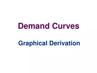
The Marshallian, Hicksian and Slutsky Demand Curves Graphical Derivation
We start with the following diagram y x px x In this part of the diagram we have drawn the choice between x on the horizontal axis and y on the vertical axis. Soon we will draw an indifference curve in here Down below we have drawn the relationship between x and its price Px. This is effectively the space in which we draw the demand curve.
Next we draw in the indifference curves showing the consumers tastes for x and y. y Then we draw in the budget constraint and find the initial equilibrium y0 x px x0
y y0 px x0 Recall the slope of the budget constraint is: x
y y0 x px x0 From the initial equilibrium we can find the first point on the demand curve Projecting x0 into the diagram below, we map the demand for x at p0x px0 x0
y y0 x px x0 px0 x0 Next consider a rise in the price of x, to px1,. This causes the budget constraint to swing in as -px1/py0 is greater To find the demand for x at the new price we locate the new equilibrium quantity of x demanded. x1 Then we drop a line down from this point to the lower diagram. px1 This shows us the new level of demand at p1x x1
y y0 x px x0 px0 x0 We are now in a position to draw the ordinary Demand Curve First we highlight the the px and x combinations we have found in the lower diagram. x1 px1 And then connect them with a line. Dx This is the Marshallian demand curve for x x1
y y0 x px x0 x1 px1 px0 Dx x1 x0 Our next exercise involves giving the consumer enough income so that they can reach their original level of utility U2 U2 So we take the new budget constraint... U1 And gradually increase the agents income, moving the budget constraint out... ...until we reach the indifference curve U2
y y0 x px x0 x1 px1 px0 Dx x1 x0 The new point of tangency tells us the demand for x when the consumer had been compensated so they can still achieve utility level U2, but the relative price of x and y has risen to px1/py0. U1
y y0 x px x0 x1 px1 px0 Dx x1 x0 The level of demand for x represents the pure substitution effect of the increase in the price of x U2 U1 This is called the Hicksian demand for x and we will label it xH xH
y y0 x px x0 x1 px1 px0 Dx x1 x0 We derive the Hicksian Demand curve by projecting the demand for x downwards into the demand curve diagram U2 U1 Notice this is the compensated demand for x when the price is px1 xH To get the Hicksian demand curve we connect the new point to the original demand x0px0 xH
y y0 x px px1 px0 Dx x1 xH x0 U2 U1 Hx We label the curve Hx Notice that the Hicksian Demand Curve is steeper than the Marshallian demand curve, when the good is a normal good
y y0 x px px1 px0 Dx x1 xH x0 Notice that an alternative compensation scheme would be to give the consumer enough income to buy their original bundle of goods, x0yo U2 In this case the budget constraint has to moved out even further until it goes through the point x0y0 x0
y y0 x px x0 px1 px0 Dx x1 xH x0 But now the consumer doesn’t have to consume x0y0 So they will choose a new equilibrium point .. On a higher indifference curve U3 U2 U1
This diagram is going to get quite messy now and I apologise for that. I could knock out the Hicksian curve to make it clearer but I want you to be able to see where it lies relative to the new one I am about to derive y U3 y0 U2 x px x0 px1 px0 Dx x1 xH x0 Once again we find the demand for x at this new higher level of income by dropping a line down from the new equilibrium point to the x axis. We call this xs . It is the Slutsky demand. xs Hx Once again this income compensated demand is measured at the price px1 xs
y U3 y0 U2 x px x0 Hx px1 px0 Dx x1 xH x0 xs Finally, once again we can draw the Slutsky compensated demand curve through this new point xspx1 and the original x0px0 Mx Sx The new demand curve Sx is steeper than either the Marshallian or the Hicksian curve when the good is normal
We can derive three demand curves on the basis of our indifference curve analysis. Summary S px H M x
1. The normal Marshallian Demand Curve S px H M x
2. The Hicksian compensated demand curve where agents are given sufficient income to maintain them on their original utility curve. S px H M x
3. The Slutsky income compensated demand curve where agents have sufficient income to purchase their original bundle S px H M x
Finally, for a normal good the Marshallian demand curve is flatter than the Hicksian, which in turn is flatter than the Slutsky demand curve. S px H M x
Problems to think about • 1) Consider the shape of the curves if x is an inferior good. • 2) Consider the shape of each of the curves x is a Giffen good. • 3) Will it matter if y is a Giffen or an inferior good?