Download

1 / 52
850 likes | 1.55k Views
Chapter 8 Slutsky Equation. Course: Microeconomics Text: Varian’s Intermediate Microeconomics. Introduction. In Chapter 6, we talk about how demand changes when price and income change individually. In this chapter, we want to further analyze how the change in price changes the demand.

E N D
Chapter 8 Slutsky Equation Course: Microeconomics Text: Varian’s Intermediate Microeconomics
Introduction • In Chapter 6, we talk about how demand changes when price and income change individually. • In this chapter, we want to further analyze how the change in price changes the demand. • In particular, we decompose the change in quantity demanded due to price change into substitution effect and income effect.
Effects of a Price Change • What happens when a commodity’s price decreases? • Substitution effect: the commodity is relatively cheaper, so consumers use more of it, instead of other commodities, which are now relatively more expensive. • Income effect: the consumer’s budget of $m can purchase more than before, as if the consumer’s income rose, with consequent income effects on quantities demanded.
Effects of a Price Change Consumer’s budget is $m. x2 Original choice x1
Effects of a Price Change Consumer’s budget is $y. x2 Lower price for commodity 1 pivots the constraint outwards. x1
Effects of a Price Change Consumer’s budget is $m. x2 Lower price for commodity 1 pivots the constraint outwards. Now only $m’ are needed to buy the original bundle at the new prices, as if the consumer’s income has increased by $m -- $m’. x1
Real Income Changes • Slutsky asserted that if, at the new prices, • If less income is needed to buy the original bundle then “real income” is increased • If more income is needed to buy the original bundle then “real income” is decreased
Effects of a Price Change • Changes to quantities demanded due to the change in relative prices, keeping income just enough to buy the original bundle, are the (pure) substitution effectof the price change. • Changes to quantities demanded due to the change in ‘real income’ are the income effect of the price change.
Effects of a Price Change • Slutsky discovered that changes to demand from a price change are always the sum of a pure substitution effect and an income effect.
Pure Substitution Effect Only x2 x2’ x1’ x1
Pure Substitution Effect Only x2 x2’ x1’ x1
Pure Substitution Effect Only x2 x2’ x1’ x1
Pure Substitution Effect Only x2 x2’ x2’’ x1’ x1’’ x1
Pure Substitution Effect Only x2 x2’ x2’’ x1’ x1’’ x1
Pure Substitution Effect Only x2 Lower p1 makes good 1 relativelycheaper and causes a substitutionfrom good 2 to good 1. (x1’,x2’) (x1’’,x2’’) is thepure substitution effect. x2’ x2’’ x1’ x1’’ x1
Pure Substitution Effect • Substitution effect is always negatively related to the price change. • Note that the portion of the yellow compensated budget line below x’1 is inside the budget set of the original budget, thus these bundles should be less preferred than the original bundle. • As a result, the consumer must choose a point at or more than x’1 with the compensated budget, and as a result, the substitution effect is positive for a price decrease.
And Now The Income Effect x2 (x1’’’,x2’’’) x2’ x2’’ x1’ x1’’ x1
And Now The Income Effect x2 The income effect is (x1’’,x2’’) (x1’’’,x2’’’). (x1’’’,x2’’’) x2’ x2’’ x1’ x1’’ x1
The Overall Change in Demand The change to demand due to lower p1 is the sum of the income and substitution effects,(x1’,x2’)(x1’’’,x2’’’). x2 (x1’’’,x2’’’) x2’ x2’’ x1’ x1’’ x1
Slutsky’s Effects for Normal Goods • Most goods are normal (i.e. demand increases with income). • The substitution and income effects reinforce each other when a normal good’s own price changes.
Slutsky’s Effects for Normal Goods x2 Good 1 is normal becausehigher income increasesdemand, so the income and substitution effects reinforce each other. (x1’’’,x2’’’) x2’ x2’’ x1’ x1’’ x1
Slutsky’s Effects for Normal Goods • Since both the substitution and income effects increase demand when own-price falls, a normal good’s ordinary demand curve slopes down. • The Law of (Downward-Sloping) Demand therefore always applies to normal goods.
Slutsky’s Effects for Inferior Goods • Some goods are inferior (i.e. demand is reduced when income is higher.) • The substitution and income effects oppose each other when an inferior good’s own price changes.
Slutsky’s Effects for Income-Inferior Goods x2 x2’ x1’ x1
Slutsky’s Effects for Income-Inferior Goods x2 x2’ x1’ x1
Slutsky’s Effects for Income-Inferior Goods x2 x2’ x1’ x1
Slutsky’s Effects for Income-Inferior Goods x2 x2’ x2’’ x1’ x1’’ x1
Slutsky’s Effects for Income-Inferior Goods x2 The pure substitution effect is as fora normal good. But, …. x2’ x2’’ x1’ x1’’ x1
Slutsky’s Effects for Income-Inferior Goods The pure substitution effect is as for a normal good. But, the income effect is in the opposite direction. x2 (x1’’’,x2’’’) x2’ x2’’ x1’ x1’’ x1
Slutsky’s Effects for Income-Inferior Goods x2 The overall changes to demand arethe sums of the substitution and income effects. (x1’’’,x2’’’) x2’ x2’’ x1’ x1’’ x1
Giffen Goods • In rare cases of extreme income-inferiority, the income effect may be larger than the substitution effect, causing quantity demanded to fall as own-price rises. • Such goods are Giffen goods.
Slutsky’s Effects for Giffen Goods x2 A decrease in p1 causes quantity demanded of good 1 to fall. x2’ x1’ x1
Slutsky’s Effects for Giffen Goods x2 A decrease in p1 causes quantity demanded of good 1 to fall. x2’’’ x2’ x1’ x1’’’ x1
Slutsky’s Effects for Giffen Goods x2 A decrease in p1 causes quantity demanded of good 1 to fall. x2’’’ x2’ x2’’ x1’ x1’’’ x1’’ x1 Substitution effect Income effect
Slutsky’s Effects for Giffen Goods • Giffen good can only result when the income effect of an inferior good is so strong that it dominates the substitution effect. • This may be possible for poor households where the low-quality necessity has taken up a large portion of expenditure. • This case is very rare, even if exists, so we have confidence that the Law of Demand almost always holds.
Mathematical Treatment • If we denote m’ as the income required to obtain the original bundle at the new prices, so thatm’=p’1 x1 + p2 x2 and m=p1 x1 + p2 x2 . • Thus the change in real income ism’– m = (p’1 – p1 ) x1 • Or
Mathematical Treatment • The substitution effect is • The Income effect is • Total Effect
Mathematical Treatment • In terms of derivative (or rate of change): • Which is known as the Slutsky Equation. • (This is just a rough presentation. The tools need for formal derivations is not covered in this class.)
Hicks Substitution Effect • Slutsky’s method of decomposition is not the only reasonable way. • Hicks proposed another way of holding “real income” constant. • Instead of compensating him to be able to buy back the original bundle, Hicks method compensates the consumer to buy back a bundle that gives him the same utility as before.
Hicks Substitution Effect • Hicks Substitution Effect is also negative, because of the convex preference. (It can also be shown by revealed preference.) • The nominal income required to maintain the utility constant is less than the one required to buy back the same bundle. It implies a larger income effect for a price decrease, but a smaller income effect for a price increase.
Income Tax vs. Quantity Tax • If government wants to impose tax to support public expenditure, or to ‘punish’ consumption of a good, say, due to pollution, various means can be used. • Here, given the revenue are the same in equilibrium, how do the effects of income tax and quantity tax on good 1 differ?(Note: Income and tax rates are regarded as given for consumers. The tax rate is adjusted so that at equilibrium the tax revenue is the same.)
Income Tax vs. Quantity Tax • Income tax corresponds to an inward shift of budget line. • Quantity tax corresponds to an inward rotation of the budget line. • When the revenues are held the same for comparison, the budget line for the income tax must pass through the optimal point for quantity tax. (Note: The tax revenue is tx1*, where x1* is the optimal quantity under quantity tax.)
Income Tax vs. Quantity Tax • With the same tax revenue, the utility level attained is higher with income tax than with the quantity tax. • But quantity tax has a stronger effect in reducing the consumption of good 1 than income tax.
Quantity Tax with Rebate • Consider a similar case. Now a tax is imposed to reduce consumption of certain good, but at the same time, an equivalent amount is rebated (given back) to the consumer. • Again, consumer has to take the rebate and tax rate constant for his decision.