Download
1 / 32
340 likes | 536 Views
Spatial structure in infectious disease epidemiology: What does it mean?. MICHAEL WARD | Faculty of Veterinary Science. A conundrum in spatial analysis. a spatial analytical framework: find show explain interesting disease patterns

E N D
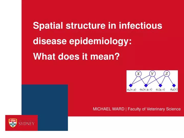
Spatial structure in infectious disease epidemiology: What does it mean? MICHAEL WARD | Faculty of Veterinary Science
A conundrum in spatial analysis • a spatial analytical framework: find show explain interesting disease patterns • assume landscape / environment determine spatial structure • inevitably confounded by the population we study Is it the environment, or is it the host population? What is the most parsimonious explanation?
Bayesian graphical network modelling A Bayesian graphical network represents the probabilistic relationships among a set of variables Equivalent to a network of multivariable generalised linear models. The joint probability distribution is encoded as a DAG (directed acyclic graph). Ref: http://www.bayesnets.com/
Bayesian graphical network modelling Structure discovery For <20 variables can use exact structure discovery methods of Koivisto & Sood (2004) As we have >20 variables, must use a heuristic approach to identify a ‘best consensus model’ Bayesian hill-climbing algorithm (Heckerman et al., 1995) vague priors placed on all nodes (covariates) and potential links (associations) Tens of thousands of searches starting from random locations in the multi-dimensional modelling space Each identifies a high scoring network structure Model averaging 50% consensus network model
Bayesian graphical network modelling multivariable confounding one outcome multivariate • Firestone, S.M., Schemann, K.A., Lewis, F.I., Ward, M.P., Toribio, J-A.L.M.L., Dhand, N.K. Modelling the associations between on-farm biosecurity practice and equine influenza infection during the 2007 outbreak in Australia. Preventive Veterinary Medicine 2013;110: 28-36 multiple inter-dependent variables 7
BGN Modelling and Spatial Analysis Case study: Salmonella infection in feral pigs
The Study Area 18.2S, 125.6E The Kimberley Fitzroy Crossing study site ~10 000 km2 Kimberley region >400 000 km2 EU: 10M km2
Salmonella distribution • 651 pigs sampled • 240 pigs Salmonella +ve(~37%) • 39 different Salmonellaserovars isolated • S. typhimurium not isolated • previous work in the EU: upper limit of prevalence
Salmonella spatial structure scan statistic (Bernoulli model) fecal–positive pigs only observed:expected 1.5
The data • faecal infection status • lymph node infection status • enhanced vegetation index 16, 32, 64, 128, 192 days • pig density • distance to a major waterway • distance to a minor waterway • distance to a waterbody • number of waterbodies • number of streams • slope • 542 observations
Multivariable and multivariate analyses • standard logistic regression (fecal, LN status separately as the outcome variable) • exact search using bootstrapping (with no parent limit) • bootstrap the dataset • find the best DAG • repeat many times until a stable majority consensus DAG obtained • exact search on the data without bootstrapping (in case above search was too conservative)
Multivariable analyses • glm(formula = LN_salmonella_pos ~ ., family = "binomial", data = mydat)Estimate Std. Error z value Pr(>|z|) (Intercept) ‒5.9819791 3.3719186 ‒1.774 0.076054 . faecal_infected1 0.9686363 0.2908965 3.330 0.000869 ***EVI_16 ‒0.0010645 0.0030285 ‒0.352 0.725211EVI_32 0.0096010 0.0078382 1.225 0.220614EVI_64 ‒0.0111865 0.0071712 ‒1.560 0.118778EVI_128 0.0079115 0.0050636 1.562 0.118186EVI_192 ‒0.0036400 0.0035296 ‒1.031 0.302422Pig_density‒3.7663023 6.6319403 ‒0.568 0.570100Dist_major_water 0.0001075 0.0002664 0.403 0.686631Dist_minor_water‒0.0227323 0.3054398 ‒0.074 0.940672Dist_waterbody‒0.0312163 0.2476048 ‒0.126 0.899674No_waterbodies 0.0665093 0.1277485 0.521 0.602627No_streams‒0.0011000 0.0461551 ‒0.024 0.980986Flat_sum 0.0025893 0.0033440 0.774 0.438757
Multivariable analyses • glm(formula = faecal_infected ~ ., family = "binomial", data = mydat)Estimate Std. Error z-value Pr(>|z|)(Intercept) 2.4726860 2.1058388 1.174 0.240313LN_salmonella_pos1 0.9904840 0.2885825 3.432 0.000599 ***EVI_16 ‒0.0004481 0.0019600 ‒0.229 0.819147EVI_32 0.0028477 0.0051640 0.551 0.581329EVI_64 ‒0.0002995 0.0038822 ‒0.077 0.938497EVI_128 ‒0.0039968 0.0032640 ‒1.224 0.220770EVI_192 0.0004255 0.0022379 0.190 0.849194Pig_density‒1.5544500 4.2949025 ‒0.362 0.717405Dist_major_water 0.0001489 0.0001691 0.880 0.378773Dist_minor_water‒0.5664415 0.1922911 ‒2.946 0.003222 ** Dist_waterbody‒0.1113402 0.1524897 ‒0.730 0.465299No_waterbodies 0.0927183 0.0802288 1.156 0.247814No_streams‒0.0350714 0.0293388 ‒1.195 0.231934Flat_sum 0.0014939 0.0023693 0.630 0.528370
Multivariable analyses distance to minor waterways LN Samonella status fecal Samonella status
stable majority consensus DAG using an exact search and boot-strapping (no parent limit) Multivariate analyses
The environment and Salmonella transmission • a relationship between distance to minor waterways and Salmonella fecal status not identified in either DAG analyses • forcing an arc into the DAG substantially reduced goodness of fit • logistic regression residuals non-Normal • identification of variable (P=0.003) probably spurious • so what drives Salmonella transmission within this environment?
How about the host population characteristics? • DICE (genetic similarity) • Salmonella status: • carrier (both pigs LN positive) • transient (≥1faecal positive) • age • gender • pregnancy status • lactation status • weight • condition • herd • pig density • 2,583 observations
Spatial structure in infectious disease epidemiology • local environment in effect a disease independent factor • simply describes the ecosystem which allows the pigs to survive • main driver of Salmonella infection is host attributes • spatial correlation does not imply spatial causation • space can be just a proxy for underlying factors such as host attributes • consider non-spatial factors first, then look for spatial explanations
Acknowledgements • Fraser Lewis, University of Zurich • Swiss National Science Foundation • Brendan Cowled, AusVet Animal Health Services • Shawn Laffan, University of New South Wales • funding: Australian Research Council • no funding: EU
Spatial structure in infectious disease epidemiology: What does it mean? MICHAEL WARD | Faculty of Veterinary Science