Download
1 / 39
400 likes | 735 Views
Chapter II: Basics from probability theory and statistics. Information Retrieval & Data Mining Universität des Saarlandes, Saarbrücken Winter Semester 2011/12. Chapter II: Basics from Probability Theory and Statistics*. II.1 Probability Theory

E N D
Chapter II:Basics from probability theory and statistics Information Retrieval & Data Mining Universität des Saarlandes, Saarbrücken Winter Semester 2011/12
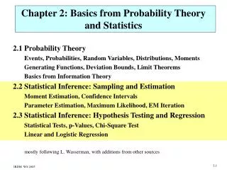
Chapter II: Basics from Probability Theoryand Statistics* • II.1 Probability Theory • Events, Probabilities, Random Variables, Distributions, Moment-Generating Functions, Deviation Bounds, Limit Theorems • Basics from Information Theory • II.2 Statistical Inference: Sampling and Estimation • Moment Estimation, Confidence Intervals • Parameter Estimation, Maximum Likelihood, EM Iteration • II.3 Statistical Inference: Hypothesis Testing and Regression • Statistical Tests, p-Values, Chi-Square Test • Linear and Logistic Regression *mostly following L. Wasserman, with additions from other sources IR&DM, WS'11/12
II.1 Basic Probability Theory • Probability Theory • Given a data generating process, what are the properties of the outcome? • Statistical Inference • Given the outcome, what can we say about the process that generated the data? • How can we generalize these observations and make predictions about future outcomes? Probability Data generating process Observed data Statistical Inference/Data Mining IR&DM, WS'11/12
Sample Spaces and Events • A sample space is a set of all possible outcomes of an experiment. (Elements e in are called sample outcomes or realizations.) • Subsets E of are called events. Example 1: • If we toss a coin twice, then = {HH, HT, TH, TT}. • The event that the first toss is heads is A = {HH, HT}. Example 2: • Suppose we want to measure the temperature in a room. • Let = R = {-∞, ∞}, i.e., the set of the real numbers. • The event that the temperature is between 0 and 23 degrees is A = [0, 23]. IR&DM, WS'11/12
Probability • A probability space is a triple (, E, P) with • a sample space of possible outcomes, • a set of events E over , • and a probability measure P: E [0,1]. Example: P[{HH, HT}] = 1/2; P[{HH, HT, TH, TT}] = 1 • Three basic axioms of probability theory: Axiom 1: P[A] ≥ 0 (for any event A in E) Axiom 2: P[] = 1 Axiom 3: If events A1, A2, … are disjoint, then P[i Ai] = i P[Ai] (for countably many Ai). IR&DM, WS'11/12
Probability More properties (derived from axioms) P[] = 0 (null/impossible event) P[] = 1 (true/certain event, actually not derived but 2nd axiom) 0 ≤ P[A] ≤ 1 If A B then P[A] ≤ P[B] P[A] + P[A] = 1 P[A B] = P[A] + P[B] – P[A B] (inclusion-exclusion principle) • Notes: • E is closed under , , and –with a countable number of operands (with finite , usually E=2). • It is not always possible to assign a probability to every event in E if the sample space is large. Instead one may assign probabilities to a limited class of sets in E. IR&DM, WS'11/12
Venn Diagrams Proof of the Inclusion-Exclusion Principle: P[A B] = P[ (A B) (A B) (A B) ] = P[A B] + P[A B] + P[A B] + P[A B] – P[A B] = P[(A B) (A B)] + P[(A B) (A B)] – P[A B] = P[A] + P[B] – P[A B] B A A B John Venn 1834-1923 IR&DM, WS'11/12
Independence and Conditional Probabilities • Two events A, B of a probability space are independent • if P[A B] = P[A] P[B]. • A finite set of events A={A1, ..., An} isindependent • if for every subset S A the equation • holds. • The conditional probabilityP[A | B] of A under the • condition (hypothesis) B is defined as: • An event A is conditionally independent of B given C • if P[A | BC] = P[A | C]. IR&DM, WS'11/12
Independence vs. Disjointness P[⌐A] = 1 – P[A] Set-Complement P[A B]= P[A] P[B] Independence P[A B] = 1 – (1 – P[A])(1 – P[B]) Disjointness P[A B]= 0 P[A B] = P[A] + P[B] P[A] = P[B] = P[A B] = P[A B] Identity IR&DM, WS'11/12
Murphy’s Law Example: • Assume a power plant has a probability of a • failure on any given day of p. • The plant may fail independently on any given • day, i.e., the probability of a failure over n days • is: P[failure in n days] = 1 – (1 – p)n Set p = 3 accidents / (365 days * 40 years) = 0.00021, then: P[failure in 1 day] = 0.00021 P[failure in 10 days] = 0.002 P[failure in 100 days] = 0.020 P[failure in 1000 days] = 0.186 P[failure in 365*40 days] = 0.950 IR&DM, WS'11/12 “Anything that can go wrong will go wrong.”
Birthday Paradox • Let N denote the event that in a group of n-1 people a newly added person does not share a birthday with any other person, then: • P[N=1] = 365/365, P[N=2]= 364/365, P[N=3] = 363/365, … • P[N’=n] = P[at least two birthdays in a group of n people coincide] • = 1 – P[N=1] P[N=2] … P[N=n-1] = 1 – ∏ k=1,…,n-1 (1 – k/365) • P[N’=1] = 0 • P[N’=10] = 0.117 • P[N’=23] = 0.507 • P[N’=41] = 0.903 • P[N’=366] = 1.0 IR&DM, WS'11/12 In a group of n people, what is the probability that at least 2 people have the same birthday? For n = 23, there is already a 50.7% probability of least 2 people having the same birthday.
Total Probability and Bayes’ Theorem The Law of Total Probability: For a partitioning of into events A1, ..., An: Thomas Bayes 1701-1761 Bayes’ Theorem: P[A|B] is called posterior probability P[A] is called prior probability IR&DM, WS'11/12
Random Variables How to link sample spaces and events to actual data/ observations? Example: Let’s flip a coin twice, and let X denote the number of heads we observe. Then what are the probabilities P[X=0], P[X=1], etc.? P[X=0] = P[{TT}] = 1/4 P[X=1] = P[{HT, TH}] = 1/4 + 1/4 = 1/2 P[X=2] = P[{HH}] = 1/4 What is the probability of P[X=3] ? Distribution of X IR&DM, WS'11/12
Random Variables • A random variable (RV) X on the probability space (, E, P) is a • function X: M with M R s.t. {e | X(e) x}E for all x M • (X is observable). Example: (Discrete RV) Let’s flip a coin 10 times, and let X denote the number of heads we observe. If e = HHHHHTHHTT, then X(e) = 7. Example: (Continuous RV) Let’s flip a coin 10 times, and let X denote the ratio between heads and tails we observe. If e = HHHHHTHHTT, then X(e) = 7/3. Example: (Boolean RV, special case of a discrete RV) Let’s flip a coin twice, and let X denote the event that heads occurs first. Then X=1 for {HH, HT}, and X=0 otherwise. IR&DM, WS'11/12
Distribution and Density Functions • FX: M [0,1] with FX(x) = P[X x] is the • cumulative distribution function (cdf) of X. • For a countable set M, the function fX: M [0,1] • with fX(x) = P[X = x] is called theprobability density function • (pdf)of X; in general fX(x) is F’X(x). • For a random variable X with distribution function F, the inverse • function F-1(q) := inf{x | F(x) > q} for q [0,1] is called quantile • function of X. • (the 0.5 quantile (aka. “50th percentile”) is called median) Random variables with countable M are called discrete, otherwise they are called continuous. For discrete random variables, the density function is also referred to as the probability mass function. IR&DM, WS'11/12
Important Discrete Distributions • Uniformdistribution over {1, 2, ..., m}: • Bernoullidistribution (single coin toss with parameter p; X: head or tail): • Binomialdistribution (coin toss n times repeated; X: #heads): • Geometricdistribution (X: #coin tosses until first head): • Poissondistribution (with rate ): • 2-Poisson mixture(with a1+a2=1): IR&DM, WS'11/12
Important Continuous Distributions • Uniform distribution in the interval [a,b] • Exponentialdistribution (e.g. time until next event of a Poisson process) • with rate = limt0 (# events in t) / t : • Hyper-exponentialdistribution: • Paretodistribution: Example of a “heavy-tailed” distribution with • Logisticdistribution: IR&DM, WS'11/12
Normal (Gaussian) Distribution • Normal distribution N(,2)(Gauss distribution; • approximates sums of independent, • identically distributed random variables): • Normal (cumulative) distribution function N(0,1): Theorem: Let X be Normal distributed with expectation and variance 2. Then is Normal distributed with expectation 0 and variance 1. Carl Friedrich Gauss, 1777-1855 IR&DM, WS'11/12
Multidimensional (Multivariate) Distributions Let X1, ..., Xm be random variables over the same probability space with domains dom(X1), ..., dom(Xm). The joint distributionof X1, ..., Xm has the density function (discrete case) (continuous case) The marginal distribution of Xi in the joint distribution of X1, ..., Xm has the density function (discrete case) (continuous case) IR&DM, WS'11/12
Important Multivariate Distributions Multinomial distribution (n, m) (n trials with m-sided dice): Multidimensional Gaussian distribution ( ): with covariance matrix with ij := Cov(Xi,Xj) (Plots from http://www.mathworks.de/) IR&DM, WS'11/12
Expectation Values, Moments & Variance For a discrete random variable X with density fX is the expectation value (mean) of X is the i-th momentof X is the variance of X For a continuous random variable X with density fX is the expectation value(mean)of X is the i-th momentof X is the variance of X Theorem: Expectation values are additive: (distributions generally not) IR&DM, WS'11/12
Properties of Expectation and Variance • E[aX+b] = aE[X]+b for constants a, b • E[X1+X2+...+Xn] = E[X1] + E[X2] + ... + E[Xn] • (i.e. expectation values are generally additive, but distributions are not!) • E[XY] = E[X]E[Y] if X and Y are independent • E[X1+X2+...+XN] = E[N] E[X] • if X1, X2, ..., XN are independent and identically distributed (iid) RVs • with mean E[X] and N is a stopping-time RV • Var[aX+b] = a2Var[X] for constants a, b • Var[X1+X2+...+Xn] = Var[X1] + Var[X2] + ... + Var[Xn] • if X1, X2, ..., Xn are independent RVs • Var[X1+X2+...+XN] = E[N] Var[X] + E[X]2Var[N] • if X1, X2, ..., XN are iid RVs with mean E[X] and variance Var[X] • and N is a stopping-time RV IR&DM, WS'11/12
Correlation of Random Variables Covarianceof random variables Xi and Xj Correlation coefficientof Xi and Xj Conditional expectation of X given Y=y (discrete case) (continuous case) IR&DM, WS'11/12
Transformations of Random Variables Consider expressions r(X,Y) over RVs, such as X+Y, max(X,Y), etc. • For each z find Az = {(x,y) | r(x,y)z} • Find cdf FZ(z) = P[r(x,y) z] = • Find pdffZ(z) = F’Z(z) Important case:Sum of independent RVs (non-negative) Z = X+Y FZ(z) = P[r(x,y) z] = “Convolution” Discrete case: IR&DM, WS'11/12
Generating Functions and Transforms X, Y, ...: continuous random variables with non-negative real values A, B, ...: discrete random variables with non-negative integer values Moment-generating function of X Generating function of A (z transform) Laplace-Stieltjes transform of A Laplace-Stieltjes transform (LST) of X Exponential: Erlang-k: Poisson: Examples: IR&DM, WS'11/12
Properties of Transforms Convolutionof independent random variables: (continuous case) (discrete case) Many more properties for other transforms, see, e.g.: L. Wasserman: All of Statistics Arnold O. Allen: Probability, Statistics, and Queueing Theory IR&DM, WS'11/12
Use Case: Score prediction for fast Top-k Queries [Theobald, Schenkel, Weikum: VLDB’04] Given: Inverted lists Li with continuous score distributions captured by independent RV’s Si Want to predict: • Consider score intervals [0, highi] at current scan positions in Li, then fi(x) = 1/highi(assuming uniform score distributions) • Convolution S1+S2is given by • But each factor is non-zero in 0 ≤ x ≤ high1and 0 ≤ z-x ≤ high2 only (for high1≤ high2), thus • Cumbersome amount of case differentiations L1 L2 L3 D10:0.8 D7 : 0.8 D21:0.7 high1 … … D4:1.0 D9 :0.9 D1:0.8 high2 … D21:0.3 … D6 :0.9 D7 :0.8 D10:0.6 high3 … D21:0.6 … IR&DM, WS'11/12
Use Case: Score prediction for fast Top-k Queries [Theobald, Schenkel, Weikum: VLDB’04] Given: Inverted lists Li with continuous score distributions captured by independent RV’s Si Want to predict: • Instead: Consider the moment-generating function for each Si • For independent Si, the moment of the convolution over all Si is given by • Apply Chernoff-Hoeffding bound on tail distribution Prune D21 if P[S2+S3 > δ] ≤ ε (using δ = 1.4-0.7 and a small confidence threshold for ε, e.g., ε=0.05) L1 L2 L3 D10:0.8 D7 : 0.8 D21:0.7 high1 … … D4:1.0 D9 :0.9 D1:0.8 high2 … D21:0.3 … D6 :0.9 D7 :0.8 D10:0.6 high3 … D21:0.6 … IR&DM, WS'11/12
Inequalities and Tail Bounds Markov inequality: P[X t] E[X] / t for t > 0 and non-neg. RV X Chebyshev inequality: P[ |XE[X]| t] Var[X] / t2 for t > 0 and non-neg. RV X Chernoff-Hoeffding bound: for Bernoulli(p) iid. RVs X1, ..., Xn and any t > 0 Corollary: for N(0,1) distr. RV Z and t > 0 Mill‘s inequality: Cauchy-Schwarz inequality: Jensen’s inequality:E[g(X)] g(E[X]) for convex function g E[g(X)] g(E[X]) for concave function g (g is convex if for all c[0,1] and x1, x2: g(cx1 + (1-c)x2) cg(x1) + (1-c)g(x2)) IR&DM, WS'11/12
Convergence of Random Variables • Let X1, X2, ... be a sequence of RVs with cdf’s F1, F2, ..., • and let X be another RV with cdf F. • Xnconverges to X in probability, XnP X, if for every > 0 • P[|XnX| > ] 0 as n • Xnconverges to X in distribution, XnD X, if • limn Fn(x) = F(x) at all x for which F is continuous • Xnconverges to X in quadratic mean, Xnqm X, if • E[(XnX)2] 0 as n • Xnconverges to X almost surely, Xnas X, if P[Xn X] = 1 Weak law of large numbers (for ) if X1, X2, ..., Xn, ... are iid RVs with mean E[X], then that is: Strong law of large numbers: if X1, X2, ..., Xn, ... are iid RVs with mean E[X], then that is: IR&DM, WS'11/12
Convergence & Approximations Theorem: (Binomial converges to Poisson) Let X be a random variable with Binomial distribution with parameters n and p := λ/n with large n and small constant λ << 1. Then Theorem: (Moivre-Laplace: Binomial converges to Gaussian) Let X be a random variable with Binomial distribution with parameters n and p. For -∞ < a ≤ b < ∞ it holds that: Φ(z) is the Normal distribution function N(0,1); a, b are integers IR&DM, WS'11/12
Central Limit Theorem Theorem: Let X1, ..., Xn be n independent, identically distributed (iid) random variables with expectation µ and variance σ2. The distribution function Fn of the random variable Zn := X1 + ... + Xn converges to a Normal distribution N(nμ, nσ2) with expectation nμ and variance nσ2. That is, for -∞ < x ≤ y < ∞ it holds that: Corollary: converges to a Normal distribution N(μ, σ2/n) with expectation μ and variance σ2/n . IR&DM, WS'11/12
Elementary Information Theory Let f(x) be the probability (or relative frequency) of the x-th symbol in some text d. The entropy of the text (or the underlying prob. distribution f) is: H(d) is a lower bound for the bits per symbol needed with optimal coding (compression). For two prob. distributions f(x) and g(x) the relative entropy (Kullback-Leibler divergence) of f to g is: Relative entropy is a measure for the (dis-)similarity of two probability or frequency distributions. It corresponds to the average number of additional bits needed for coding information (events) with distribution f when using an optimal code for distribution g. The cross entropyof f(x) to g(x) is: IR&DM, WS'11/12
Compression • Text is sequence of symbols (with specific frequencies) • Symbols can be • letters or other characters from some alphabet Σ • strings of fixed length (e.g. trigrams, “shingles”) • or words, bits, syllables, phrases, etc. Limits of compression: Let pi be the probability (or relative frequency) of the i-th symbol in text d Then the entropy of the text: is a lower bound for the average number of bits per symbol in any compression (e.g. Huffman codes) Note: Compression schemes such as Ziv-Lempel (used in zip) are better because they consider context beyond single symbols; with appropriately generalized notions of entropy, the lower-bound theorem does still hold. IR&DM, WS'11/12
Summary of Section II.1 • Bayes’ Theorem: very simple, very powerful • RVs as a fundamental, sometimes subtle concept • Rich variety of well-studied distribution functions • Moments and moment-generating functions capture distributions • Tail boundsuseful for non-tractable distributions • Normal distribution: limit of sum of iid RVs • Entropymeasures (incl. KL divergence) • capture complexity and similarity of prob. distributions IR&DM, WS'11/12
Reference Tables on Probability Distributions and Statistics (1) Source: Arnold O. Allen, Probability, Statistics, and Queueing Theory with Computer Science Applications, Academic Press, 1990 IR&DM, WS'11/12
Reference Tables on Probability Distributions and Statistics (2) Source: Arnold O. Allen, Probability, Statistics, and Queueing Theory with Computer Science Applications, Academic Press, 1990 IR&DM, WS'11/12
Reference Tables on Probability Distributions and Statistics (3) Source: Arnold O. Allen, Probability, Statistics, and Queueing Theory with Computer Science Applications, Academic Press, 1990 IR&DM, WS'11/12
Reference Tables on Probability Distributions and Statistics (4) Source: Arnold O. Allen, Probability, Statistics, and Queueing Theory with Computer Science Applications, Academic Press, 1990 IR&DM, WS'11/12