DFT and Convolution

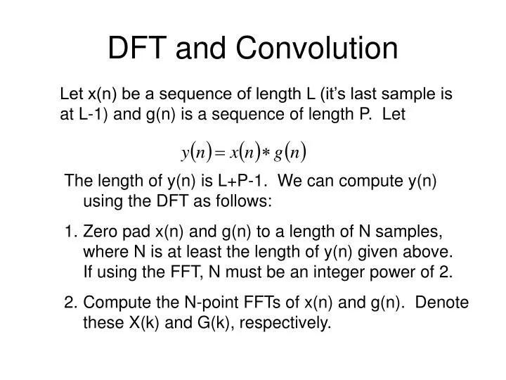
1. DFT and Convolution Let x(n) be a sequence of length L (it’s last sample is at L-1) and g(n) is a sequence of length P. Let • The length of y(n) is L+P-1. We can compute y(n) using the DFT as follows: • Zero pad x(n) and g(n) to a length of N samples, where N is at least the length of y(n) given above. If using the FFT, N must be an integer power of 2. • Compute the N-point FFTs of x(n) and g(n). Denote these X(k) and G(k), respectively.

2. DFT and Convolution • Multiply X(k) and G(k), point-by-point. Denote the result Y(k). • Compute the inverse N-point of Y(k) to obtain y(n).

3. DFT and Convolution If we wish to use fast convolution to filter a signal continuously streaming through a process (greater than N samples in length), it must be divided into subsequences of N samples which are processed individually and then reassembled. The techniques for reassembling them are called overlap-save and overlap-add. Cartinhour mentions these, but does not explain how they work or how they are used. I may present an example later in the semester, if time permits

4. Problems

5. A DSP Chip The Analog Devices ADSP-2181 We’re finally going to take a look at how a Digital Signal Processor chip works, and how to use it. First, though, let’s take a look at a general purpose microprocessor, and why it’s not very suitable for DSP applications

6. A DSP Chip Here’s the architecture of a first-generation, von Neumann processor: Data Bus TMP. Data Instruction. Registers ALU. Memory (Program and Data) Accum. Prog. Cntr Addr. Reg. Address Address Bus Control & Timing

7. A DSP Chip • Notice that the von Neumann processor has one memory space which is used for both program and data. • It has one data bus, and one address bus. • To execute an instruction, do the following: • Fetch the instruction. • If an operand is needed, fetch it. • If a second operand is needed, fetch it. • Perform the operation • Write the result to memory.

8. A DSP Chip This worst-case, two-operand instructions requires 5 cycles, and must access memory four times. This limits throughput, which is very important in DSP Using a single memory space for both program and data causes a bottleneck. One way of speeding things up is to separate the program memory from the data memory

9. A DSP Chip Data Bus Instruction Bus Instruction. Computation Unit Data Memory Program Memory Sequencer Address DAG Address Data. Addr Prog. Addr

10. A DSP Chip This is called Harvard architecture An instruction and an operand may be fetched at the same time. A result can be written to Data Memory while the next instruction is being fetched from Program Memory The DAG (Data Address Generator) calculates addresses, which would have been done by the ALU. This reduces the load on the computation unit. The architecture of a DSP chip is optimized for executing an algorithm repeatedly, very fast.

11. A DSP Chip A top-level block diagram of the 2181 is shown on the next slide. Note that in addition to an ALU, it has a dedicated Multiplier/Accumulator (MAC) for multiplying data samples by weighting factors, and a dedicated shifter for scaling data to prevent overflow and underflow It also has two Data Address Generators, which are useful for implementing circular buffers.

13. A DSP Chip Some example code – an FIR filter /*ADSP-2181 FIR Filter Routine -serial port 0 used for I/O -internally generated serial clock -40.000 MHz processor clock rate is divided to generate a 1.5385 MHz serial clock -serial clock divided to 8 kHz frame sampling rate*/ #include <def2181.h> #define taps 15 #define taps_less_one 14 .section/dm dm_data; .var/circ data_buffer[taps]; /* dm data buffer */

14. A DSP Chip /* The following lines set up a circular buffer in data memory, which is used as a delay line of samples */ . section/dm dm_data; .var/circ data_buffer[taps]; /* dm data buffer */ /* This section sets up a circular buffer in program memory which will hold the filter coefficients. The data width is 24 bits. This buffer is loaded from the named file by the linker. */ section/pm pm_data; .var/circ/init24 coefficient[taps] = "coeff.dat";

15. A DSP Chip /* The following lines of code set up the interrupt table. */ .section/pm Interrupts; start: jump main; rti; rti; rti; /* 0x0000: ~Reset vector */ rti; rti; rti; rti; /* 0x0004: ~IRQ2 */ rti; rti; rti; rti; ‘ /* 0x0008: ~IRQL1 */ rti; rti; rti; rti; /* 0x000c: ~IRQL0 */ rti; rti; rti; rti; /* 0x0010: SPORT0 Transmit */ jump fir_start; rti; rti; rti; /* 0x0014: SPORT0 Receive */ rti; rti; rti; rti; /* 0x0018: ~IRQE */ rti; rti; rti; rti; /* 0x001c: BDMA */ rti; rti; rti; rti; /* 0x0020: SPORT1 Transmit or ~IRQ1 */ rti; rti; rti; rti; /* 0x0024: SPORT1 Receive or ~IRQ0 */ rti; rti; rti; rti; /* 0x0028: Timer */ rti; rti; rti; rti; /* 0x002c: Power Down (non-maskable) */

16. A DSP Chip /* This portion of the code sets up the DAG registers for the two circular buffers */ .section/pm pm_code; main: l0 = length (data_buffer); /* setup circular buffer length */ l4 = length (coefficient); /*setup circular buffer */ m0 = 1; /* modify =1 for increment */ m4 = 1; /* through buffers */ i0 = data_buffer; /* point to start of buffer */ i4 = coefficient; /* point to start of buffer */ ax0 = 0; cntr = length(data_buffer); /* initialize loop counter */ do clear until ce; clear: dm(i0,m0) = ax0; /* clear data buffer */

17. A DSP Chip /* This slide and the next contain code which sets up the control registers. The following lines set up the internal serial clock, and the receive frame sync rate. */ /* setup divide value for 8KHz RFS*/ ax0 = 0x00c0; dm(Sport0_Rfsdiv) = ax0; /* 1.5385 MHz internal serial clock */ ax0 = 0x000c; dm(Sport0_Sclkdiv) = ax0;

18. A DSP Chip /* more control register setup */ /* multichannel disabled, internally generated sclk, receive frame sync required, receive width = 0, transmit frame sync required, transmit width = 0, external transmit frame sync, internal receive frame sync,u-law companding, 8-bit words */ ax0 = 0x69b7; dm(Sport0_Ctrl_Reg) = ax0; ax0 = 0x1000; /* enable sport0 */ dm(Sys_Ctrl_Reg) = ax0; icntl = 0x00; /* disable interrupt nesting */ imask = 0x0060; /* enable sport0 rx and tx interrupts only */

19. A DSP Chip /* The processor will sit in this loop, until data is received from SPORT0 */ mainloop: idle; /* wait here for interrupt */ jump mainloop; /* jump back to idle after rti */

20. A DSP Chip fir_start: si = rx0; /* read from sport0 */ dm(i0,m0) = si; /* transfer data to buffer */ mr = 0, my0 = pm(i4,m4), mx0 = dm(i0,m0); /* setup multiplier for loop */ cntr = taps_less_one; /* perform loop taps-1 times */ do convolution until ce; convolution: mr = mr + mx0 * my0 (ss), my0 = pm(i4,m4), mx0 = dm(i0,m0); /* perform MAC and fetch next values */ mr = mr + mx0 * my0 (rnd); /* Nth pass of loop with rounding of result */ if mv sat mr; tx0 = mr1; /* write result to sport0 tx */ rti; /* return from interrupt */

21. A DSP Chip Highly Recommended: Read Chapter 2 of the ADSP-218x DSP Instruction Set Reference

22. FIR Filter Design We’ve seen how to design a simple FIR lowpass filter using a rectangular window. • We will now see how to design lowpass, highpass, bandpass and band-reject (bandstop) filters using two techniques: • The Kaiser window (a “better” window than the rectangular window • The Parks-McClellan algorithm

23. FIR Filter Design Both methods result in filters which have linear phase characteristics: Where A(w) is a real-valued function, and N is the length of the impulse response. Within the passband, A(w) is real and nonnegative. This means the resulting filter has linear phase, not merely general linear phase

24. FIR Filter Design Within the passband, A(w) is real and nonnegative. This means the resulting filter has linear phase, not merely general linear phase. These equations apply: Outside the passband, the filter may have jump discontinuities in its phase characteristic (general linear phase), but since this isoutside the passband, they have little significance.

25. The Window Method We’ve seen how to design lowpass filters using a rectangular window. The rectangular window truncates the impulse response to a length of N samples.

26. The Window Method Here’s another way of writing the impulse response: Where wc is the cutoff frequency, and w(n) is the rectangular window function.

27. The Window Method The window function is: The frequency response of the resulting filter can be written:

28. The Window Method The frequency response of the resulting filter can be written: W(ejw) is the DTFT of the rectangular window, and Hi(ejw) is the frequency response function of the ideal lowpass filter.

29. The Window Method When this convolution is performed, the shape of the main lobe and sidelobes of W(ejw) modify the shape of the frequency response. Instead of being rectangular, the frequency response has ripple in the passband and the stopband.

31. The Window Method It would be good to reduce the amount of ripple. Maybe this can be done by using a window who’s shape is different. In particular, if the window’s DTFT has sidelobes which are smaller in magnitude relative to the mainlobe, the ripple will be reduced. A “tapered” window will have smaller sidelobes, and a wider main lobe – both desirable characteristics.

32. The Window Method As an example, here’s the Hamming window: A 29-point Hamming window is plotted on the next slide

34. The Window Method Next, a plot of the impulse response of a 29-tap FIR lowpass filter, wc = 0.46p, based on an ideal lowpass, followed by it’s frequency response Note the magnitude of the impulse response’s sidelobes, and the passband ripple

37. The Window Method The next plot is the impulse response shown previously, but windowed by a Hamming window. This is followed by the filter’s frequency response. Note the reduced sidelobe magnitude, and the reduced passband ripple However, the transition from passband to stopband is not as sharp. The sharpness can be restored by increasing the filter length.

40. The Window Method The Hamming window tapers the impulse response. Other windows taper the impulse response more, or less, than the Hamming window. The rectangular window is an extreme example: it tapers the impulse response LESS!! A window which tapers more will have a wider main lobe (less sharp transition), but smaller sidelobes (less ripple).

41. The Window Method If we’re given a filter specification, it will usually include the cutoff frequency. This may be wc (radians per sample) or fs (Hertz). It will also give the width of the transition band, and the minimum stopband attenuation. We must choose the window function, and the filter length in order to meet the specification.