Download
1 / 71
730 likes | 747 Views
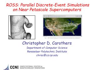
Christopher D. Carothers Department of Computer Science Rensselaer Polytechnic Institute chrisc@cs.rpi.edu. Parallel Discrete-Event Simulations. Motivation. Why Parallel Discrete-Event Simulation (DES)? Large-scale systems are difficult to understand

E N D
Christopher D. Carothers Department of Computer Science Rensselaer Polytechnic Institute chrisc@cs.rpi.edu Parallel Discrete-Event Simulations
Motivation Why Parallel Discrete-Event Simulation (DES)? • Large-scale systems are difficult to understand • Analytical models are often constrained Parallel DES simulation offers: • Dramatically shrinks model’s execution-time • Prediction of future “what-if” systems performance • Potential for real-time decision support • Minutes instead of days • Analysis can be done right away • Example models: national air space (NAS), ISP backbone(s), distributed content caches, next generation supercomputer systems.
Ex: Movies over the Internet • Suppose we want to model 1 million home ISP customers downloading a 2 GB movie • How long to compute? • Assume a nominal 100K ev/sec seq. simulator • Assume on avg. each packet takes 8 hops • 2GB movies yields 2 trillion 1K data packets. • @ 8 hops yields 16+ trillion events • 16+ trillion events @ 100K ev/sec • Over 1,900 days!!! Or • 5+ years!!! • Need massively parallel simulation to make tractable
Outline • Intro to DES • Time Warp and other PDES Schemes • Reverse Computation • Blue Gene/L & /P • ROSS Implementation • ROSS Performance Results • PHOLD & PCS • Observations on PDES Performance • Future Directions
Discrete Event Simulation (DES) • Discrete event simulation: computer model for a system where changes in the state of the system occur at discrete points in simulation time. • Fundamental concepts: • system state (state variables) • state transitions (events) • A DES computation can be viewed as a sequence of event computations, with each event computation is assigned a (simulation time) time stamp • Each event computation can • modify state variables • schedule new events
processed event current event unprocessed event DES Computation example: air traffic at an airport events: aircraft arrival, landing, departure • Unprocessed events are stored in a pending list • Events are processed in time stamp order arrival 8:00 schedules departure 9:15 arrival 9:30 landed 8:05 schedules simulation time
Simulation Application • state variables • code modeling system behavior • I/O and user interface software calls to schedule events calls to event handlers • Simulation Executive • event list management • managing advances in simulation time Discrete Event Simulation System model of the physical system independent of the simulation application
Simulation executive • Event processing loop While (simulation not finished) E = smallest time stamp event in PEL Remove E from PEL Now := time stamp of E call event handler procedure Now = 8:45 Pending Event List (PEL) 9:00 10:10 9:16 Event-Oriented World View • Event handler procedures state variables Departure Event { … } Arrival Event { … } Landed Event { … } Integer: InTheAir; Integer: OnTheGround; Boolean: RunwayFree; Simulation application
Ex: Air traffic at an Airport Model aircraft arrivals and departures, arrival queueing Single runway model; ignores departure queueing • R = time runway is used for each landing aircraft (const) • G = time required on the ground before departing (const) State Variables • Now: current simulation time • InTheAir: number of aircraft landing or waiting to land • OnTheGround: number of landed aircraft • RunwayFree: Boolean, true if runway available • Model Events • Arrival: denotes aircraft arriving in air space of airport • Landed: denotes aircraft landing • Departure: denotes aircraft leaving
Arrival Events New aircraft arrives at airport. If the runway is free, it will begin to land. Otherwise, the aircraft must circle, and wait to land. • R = time runway is used for each landing aircraft • G = time required on the ground before departing • Now: current simulation time • InTheAir: number of aircraft landing or waiting to land • OnTheGround: number of landed aircraft • RunwayFree: Boolean, true if runway available Arrival Event: InTheAir := InTheAir+1; If (RunwayFree) RunwayFree:=FALSE; Schedule Landed event @ Now + R;
Landed Event An aircraft has completed its landing. • R = time runway is used for each landing aircraft • G = time required on the ground before departing • Now: current simulation time • InTheAir: number of aircraft landing or waiting to land • OnTheGround: number of landed aircraft • RunwayFree: Boolean, true if runway available Landed Event: InTheAir:=InTheAir-1; OnTheGround:=OnTheGround+1; Schedule Departure event @ Now + G; If (InTheAir>0) Schedule Landed event @ Now + R; Else RunwayFree := TRUE;
Departure Event An aircraft now on the ground departs for a new dest. • R = time runway is used for each landing aircraft • G = time required on the ground before departing • Now: current simulation time • InTheAir: number of aircraft landing or waiting to land • OnTheGround: number of landed aircraft • RunwayFree: Boolean, true if runway available Departure Event: OnTheGround := OnTheGround - 1;
State Variables R=3 G=4 InTheAir 0 1 1 0 2 1 0 OnTheGround 0 1 2 RunwayFree true false true 0 1 2 3 4 5 6 7 8 9 10 11 Simulation Time Processing: Arrival F1 Arrival F2 Landed F1 Landed F2 Depart F1 Depart F2 Time Event Time Event Time Event Time Event Time Event Time Event Time Event 1 Arrival F1 3 Arrival F2 3 Arrival F2 4 Landed F1 4 Landed F1 7 Landed F2 8 Depart F1 8 Depart F1 11 Depart F2 11 Depart F2 Now=0 Now=1 Now=3 Now=4 Now=7 Now=8 Now=11 Execution Example
Summary • DES computation is sequence of event computations • Modify state variables • Schedule new events • DES System = model + simulation executive • Data structures • Pending event list to hold unprocessed events • State variables • Simulation time clock variable • Program (Code) • Main event processing loop • Event procedures • Events processed in time stamp order
Outline • Intro to DES • Time Warp and other PDES Schemes • Reverse Computation • Blue Gene/L & /P • ROSS Implementation • ROSS Performance Results • PHOLD & PCS • Observations on PDES Performance • Future Directions
parallel time-stepped simulation: lock-step execution parallel discrete-event simulation: must allow for sparse, irregular event computations barrier Problem: events arriving in the past Solution: Time Warp Virtual Time Virtual Time PE 2 PE 3 PE 1 PE 2 PE 3 PE 1 How to Synchronize Parallel Simulations? processed event “straggler” event
Massively Parallel Discrete-Event Simulation Via Time Warp Local Control Mechanism: error detection and rollback Global Control Mechanism: compute Global Virtual Time (GVT) V i r t u a l T i m e V i r t u a l T i m e collect versions of state / events & perform I/O operations that are < GVT (1) undo state D’s (2) cancel “sent” events GVT LP 2 LP 3 LP 1 LP 2 LP 3 LP 1 unprocessed event processed event “straggler” event “committed” event
Whew …Time Warp sounds expensive are there other PDES Schemes?… • “Non-rollback” options: • Called “Conservative” because they disallow out of order event execution. • Deadlock Avoidance • NULL Message Algorithm • Deadlock Detection and Recovery
Deadlock Avoidance Using Null Messages Null Message Algorithm (executed by each LP): Goal: Ensure events are processed in time stamp order and avoid deadlock WHILE (simulation is not over) wait until each FIFO contains at least one message remove smallest time stamped event from its FIFO process that event send null messages to neighboring LPs with time stamp indicating a lower bound on future messages sent to that LP (current time plus minimum transit time between airports) END-LOOP • Variation: LP requests null message when FIFO becomes empty • Fewer null messages • Delay to get time stamp information
7 7 ORD (waiting on SFO) Null messages: 6.0 JFK: timestamp = 5.5 7.5 SFO: timestamp = 6.0 6.5 ORD: timestamp = 6.5 JFK (waiting on ORD) 15 JFK: timestamp = 7.0 7.0 5.5 10 SFO (waiting on JFK) SFO: timestamp = 7.5 9 8 ORD: process time stamp 7 message 0.5 Assume minimum delay between airports is 3 units of time JFK initially at time 5 The Time Creep Problem Many null messages if minimum flight time is small! Five null messages to process a single event!
ORD (waiting on SFO) 7 JFK (waiting on ORD) 15 10 SFO (waiting on JFK) 9 8 Livelock Can Occur! Suppose the minimum delay between airports is zero! 5.0 5.0 5.0 5.0 Livelock: un-ending cycle of null messages where no LP can advance its simulation time There cannot be a cycle where for each LP in the cycle, an incoming message with time stamp T results in a new message sent to the next LP in the cycle with time stamp T (zero lookahead cycle)
Lookahead The null message algorithm relies on a “prediction” ability referred to as lookahead • “ORD at simulation time 5, minimum transit time between airports is 3, so the next message sent by ORD must have a time stamp of at least 8” Lookahead is a constraint on LP’s behavior • Link lookahead: If an LP is at simulation time T, and an outgoing link has lookahead Li, then any message sent on that link must have a time stamp of at least T+Li • LP Lookahead: If an LP is at simulation time T, and has a lookahead of L, then any message sent by that LP must will have a time stamp of at least T+L • Equivalent to link lookahead where the lookahead on each outgoing link is the same
Lookahead and the Simulation Model Lookahead is clearly dependent on the simulation model • could be derived from physical constraints in the system being modeled, such as minimum simulation time for one entity to affect another (e.g., a weapon fired from a tank requires L units of time to reach another tank, or maximum speed of the tank places lower bound on how soon it can affect another entity) • could be derived from characteristics of the simulation entities, such as non-preemptable behavior (e.g., a tank is traveling north at 30 mph, and nothing in the federation model can cause its behavior to change over the next 10 minutes, so all output from the tank simulator can be generated immediately up to time “local clock + 10 minutes”) • could be derived from tolerance to temporal inaccuracies (e.g., users cannot perceive temporal difference of 100 milliseconds, so messages may be timestamped 100 milliseconds into the future). • simulations may be able to precompute when its next interaction with another simulation will be (e.g., if time until next interaction is stochastic, pre-sample random number generator to determine time of next interaction). Lookahead changes as LP topology changes which can have a profound impact on the performance of network models (wired or wireless).
problem: limited concurrency each LP must process events in time stamp order event without lookahead LP D possible message OK to process LP C with lookahead possible message LP B OK to process LP A not OK to process yet LTA+LA LTA Logical Time Why is Lookahead Important? Each LP A using logical time declares a lookahead value LA; the time stamp of any event generated by the LP must be ≥ LTA+ LA • Lookahead is used in virtually all conservative synch. protocols • Essential to allow concurrent processing of events Lookahead is necessary to allow concurrent processing of events with different time stamps (unless optimistic event processing is used)
Null Message Algorithm: Speed Up • toroid topology • message density: 4 per LP • 1 millisecond computation per event • vary time stamp increment distribution • ILAR=lookahead / average time stamp increment Conservative algorithms live or die by their lookahead!
Deadlock Detection & Recovery Algorithm A (executed by each LP): Goal: Ensure events are processed in time stamp order: WHILE (simulation is not over) wait until each FIFO contains at least one message remove smallest time stamped event from its FIFO process that event END-LOOP • No null messages • Allow simulation to execute until deadlock occurs • Provide a mechanism to detect deadlock • Provide a mechanism to recover from deadlocks
ORD (waiting on SFO) 7 deadlock state Assume minimum delay between airports is 3 JFK (waiting on ORD) 10 SFO (waiting on JFK) 9 8 Deadlock Recovery Deadlock recovery: identify “safe” events (events that can be processed w/o violating local causality), • Which events are safe? • Time stamp 7: smallest time stamped event in system • Time stamp 8, 9: safe because of lookahead constraint • Time stamp 10: OK if events with the same time stamp can be processed in any order • No lookahead creep!
ORD (waiting on SFO) 7 JFK (waiting on ORD) 15 10 SFO (waiting on JFK) 9 8 Preventing LA Creep Using Next Event Time Info Observation: smallest time stamped event is safe to process • Lookahead creep avoided by allowing the synchronization algorithm to immediately advance to (global) time of the next event • Synchronization algorithm must know time stamp of LP’s next event • Each LP guarantees a logical time T such that if no additional events are delivered to LP with TS < T, all subsequent messages that LP produces have a time stamp at least T+L (L = lookahead)
No Free Lunch for PDES! • Time Warp State saving overheads • Null message algorithm Lookahead creep problem • No zero lookahead cycles allowed • Lookahead Essential for concurrent processing of events for conservative algorithms • Has large effect on performance need to program it • Deadlock Detection and Recovery Smallest time stamp event safe to process • Others may also be safe (requires additional work to determine this) • Use time of next event to avoid lookahead creep, but hard to compute at scale… Can we avoid some of these overheads and complexities??
Outline • Intro to DES • Time Warp and other PDES Schemes • Reverse Computation • Blue Gene/L & /P • ROSS Implementation • ROSS Performance Results • PHOLD & PCS • Observations on PDES Performance • Future Directions
Our Solution: Reverse Computation... • Use Reverse Computation (RC) • automatically generate reverse code from model source • undo by executing reverse code • Delivers better performance • negligible overhead for forward computation • significantly lower memory utilization Original Code Compiler Modified Code Reverse Code
Forward Reverse if( qlen < B ) b1 = 1 qlen++ delays[qlen]++ else b1 = 0 lost++ if( b1 == 1 ) delays[qlen]-- qlen-- else lost-- Ex: Simple Network Switch Original N if( qlen < B ) qlen++ delays[qlen]++ else lost++ B on packet arrival...
Benefits of Reverse Computation • State size reduction • from B+2 words to 1 word • e.g. B=100 => 100x reduction! • Negligible overhead in forward computation • removed from forward computation • moved to rollback phase • Result • significant increase in speed • significant decrease in memory • How?...
Beneficial Application Properties • 1. Majority of operations are constructive • e.g., ++, --, etc. • 2. Size of control state< size of data state • e.g., size of b1 < size of qlen, sent, lost, etc. • 3. Perfectly reversible high-level operations • gleaned from irreversible smaller operations • e.g., random number generation
Rules for Automation... Generation rules, and upper-bounds on bit requirements for various statement types
Destructive Assignment... • Destructive assignment (DA): • examples: x = y; x %= y; • requires all modified bytes to be saved • Caveat: • reversing technique forDA’s can degenerate to traditional incremental state saving • Good news: • certain collections of DA’s are perfectly reversible! • queueing network models contain collections of easily/perfectly reversible DA’s • queue handling (swap, shift, tree insert/delete, … ) • statistics collection (increment, decrement, …) • random number generation (reversible RNGs)
Reversing an RNG? double RNGGenVal(Generator g) { long k,s; double u; u = 0.0; s = Cg [0][g]; k = s / 46693; s = 45991 * (s - k * 46693) - k * 25884; if (s < 0) s = s + 2147483647; Cg [0][g] = s; u = u + 4.65661287524579692e-10 * s; s = Cg [1][g]; k = s / 10339; s = 207707 * (s - k * 10339) - k * 870; if (s < 0) s = s + 2147483543; Cg [1][g] = s; u = u - 4.65661310075985993e-10 * s; if (u < 0) u = u + 1.0; s = Cg [2][g]; k = s / 15499; s = 138556 * (s - k * 15499) - k * 3979; if (s < 0.0) s = s + 2147483423; Cg [2][g] = s; u = u + 4.65661336096842131e-10 * s; if (u >= 1.0) u = u - 1.0; s = Cg [3][g]; k = s / 43218; s = 49689 * (s - k * 43218) - k * 24121; if (s < 0) s = s + 2147483323; Cg [3][g] = s; u = u - 4.65661357780891134e-10 * s; if (u < 0) u = u + 1.0; return (u); } Observation: k = s / 46693 is a Destructive AssignmentResult: RC degrades to classic state-saving…can we do better?
RNGs: A Higher Level View The previous RNG is based on the following recurrence…. xi,n = aixi,n-1 mod mi where xi,none of the four seed values in the Nth set, miis one the four largest primes less than 231, and ai is a primitive root of mi. Now, the above recurrence is in fact reversible…. inverse of aimodulo mi is defined, bi = aimi-2 mod mi Using bi, we can generate the reverse recurrence as follows: xi,n-1 = bixi,n mod mi
Reverse Code Efficiency... • Property... • Non-reversibility of indvidual steps DO NOT imply that the computation as a whole is not reversible. • Can we automatically find this “higher-level” reversibility? • Other Reversible Structures Include... • Circular shift operation • Insertion & deletion operations on trees (i.e., priority queues). Reverse computation is well-suited for small grain event models!
Original if( qlen < B ) qlen++ delays[qlen]++ else lost++ B packet arrival... Forward Reverse if( qlen < B ) b1 = 1 qlen++ delays[qlen]++ else b1 = 0 lost++ if( b1 == 1 ) delays[qlen]-- qlen-- else lost-- RC Applications • PDES applications include: • Wireless telephone networks • Distributed content caches • Large-scale Internet models – • TCP over AT&T backbone • Leverges RC “swaps” • Hodgkin-Huxley neuron models • Plasma physics models using PIC • Non-DES include: • Debugging • PISA – Reversible instruction set architecture for low power computing • Quantum computing
Outline • Intro to DES • Time Warp and other PDES Schemes • Reverse Computation • Blue Gene/L & /P • ROSS Implementation • ROSS Performance Results • PHOLD & PCS • Observations on PDES Performance • Future Directions
Target Systems: Blue Gene/L & /P • Configuration: • BG/L nodes: 2x700 MHz PPC cores • BG/P nodes: 4x850 MHz PPC cores • Dediciated compute and I/O nodes (32:1 or 8:1). • 3-D torus P2P network • Additional barrier, collective, I/O and ethernet networks • Can partition system into dedicated slices from 32 nodes to whole systems • Properties for GOOD scaling: • Balanced architecture between network(s) and processor speed • Exclusive access to network and process • Exceptionally low OS jitter • Collective overheads not adversely impacted at large nodes counts 1 rack of IBM Blue Gene/L
Blue Gene/P Architectual Highlights • Scaled performance via density and frequency increase • 2x performance increase via doubling the processors per node. • 1.2x from frequency increase: 700 MHz 850 MHz. • Enhanced function • 4-way SMP 3 modes: SMP/ DUAL/ VNM • L2, L3 changed for SMP mode • DMA for torus, remote put-get, user prog. memory prefetch • Enhanced 64-bit performance counters via PPC450 core • Double Hummer FPU and networks are the same..except.. • Better Network • 2.4x more bandwidth, lower latency Torus and Tree neworks • 10x higher Ethernet I/O bandwidth • 72K nodes in 72 racks for 1 PF peak performance • Low power via aggressive power management
Outline • Intro to DES • Time Warp and other PDES Schemes • Reverse Computation • Blue Gene/L & /P • ROSS Implementation • ROSS Performance Results • PHOLD & PCS • Observations on PDES Performance • Future Directions