Download
1 / 50
510 likes | 1.12k Views
Fourier Domain OCT: The RTVue. Michael J. Sinai, PhD Director of Clinical Affairs Optovue, Inc. Rise of Structural Assessment with Scanning Lasers . Scanning lasers provide objective and quantitative information for numerous ocular pathologies

E N D
Fourier Domain OCT: The RTVue Michael J. Sinai, PhD Director of Clinical Affairs Optovue, Inc.
Rise of Structural Assessment with Scanning Lasers • Scanning lasers provide objective and quantitative information for numerous ocular pathologies • First appeared over 20 years ago as a research tool • Today, structural assessment with retinal imaging devices has become an indispensable tool for clinicians
Role of imaging in clinical practice • AAO preferred practice patterns recommends using scanning laser imaging in routine clinical exams • In glaucoma, studies show imaging results can be as good as expert grading of high quality stereo-photographs1 • Pre-perimetric glaucoma is now commonly accepted • In OHTS, most converted based on structural assessment only (not fields) 2 • OHTS has shown that imaging results have a high positive and negative predictive power for detecting glaucoma 3 • Wollstein et al. Ophthalmology 2000 • Kass et al. Arch Ophthalmol 2001 • Zangwill LM, Weinreb RN, et al. Archives of Ophthalmol. 2005.
3 Imaging technologies have been shown to be effective in detecting and managing ocular pathologies Light Polarizer • Scanning Laser Polarimetry (SLP) • Confocal Scanning Laser Ophthalmoscopy (CSLO) • Optical Coherence Tomography (OCT) Two polarized components Birefringent structure (RNFL) Retardation
SLP – GDx VCC • Strengths • Provides RNFL thickness • Large database • Easy to use/interpret (deviation map/automated classifier) • Progression • Weaknesses • Atypical Pattern Birefringence (RNFL artifact)1 • Converts retardation to thickness assuming uniform birefringence (not true) 2 • Only RNFL information (No Optic Disc info and no Retina info) • Data not backwards compatible Normal Glaucoma Atypical 1. Bagga, Greenfield, Feuer. AJO, 2005: 139: 437. 2. Huang, Bagga, Greenfield, Knighton IOVS, 2004: 45: 3037.
CSLO – HRT 3 • Strengths • Provides Optic Disc morphology • Sophisticated Progression Analysis • Large ethnic Specific Database comparisons • Automated classifier • Data backwards compatible • Some retinal capabilities • Cornea microscope attachment • Weaknesses • Only Optic Disc assessment (poor RNFL) • Manual Contour Line drawing • Reference plane based on surface height (can change) • Retina analysis confined to edema detection and sensitive to image quality • Cornea scans very difficult and impractical
OCT – Time Domain (Stratus from CZM and SLO/OCT from OTI) • Strengths • Provides Cross Sectional images • Useful to calculate RNFL thickness • Cross section scans useful for retinal pathologies • Database comparisons • Weaknesses • Slow scan speed (400 A scans / second) • Limited data for glaucoma, 768 pixel (A-scan) ring for RNFL • Limited data for retina, 6 radial lines with 128 A scans (pixels) each • Macula maps 97% interpolated • No progression analysis • Location of scan ring affects RNFL results • Prone to motion artifacts because of slow scan speed • Poor optic disc measurements
Time Domain OCT susceptible to eye movements • 768 pixels (A-scans) captured in 1.92 seconds is slower than eye movements • Stabilizing the retina reveals true scan path (white circles)1 1. Koozekanani, Boyer and Roberts. “Tracking the Optic Nervehead in OCT Video Using Dual Eigenspaces and an Adaptive Vascular Distribution Model”; IEEE Transactions on Medical Imaging, Vol. 22, No. 12, 2003
Scan location and eye movements affects results Properly centered Poorly centered: too inferior Poorly centered: too superior T S N I T T S N I T T S N I T Superior RNFL “Loss” Inferior RNFL “Loss” Normal Double Hump
Time Domain OCT artifacts can be common • Sadda, Wu, et al. Ophthalmology 2006;113:285-293 • Ray, Stinnett, Jaffe . Am J Ophth 2005; 139:18-29 • Bartsch, Gong, et al. Proc. of SPIE Vol. 5370; 2140-2151
The Future of OCT • RTVue Fourier Domain OCT overcomes limitations of Time Domain OCT Devices • Better resolution (5 micron VS 10 micron) • Faster scan speeds (26,000 A scans / sec VS 400) • 3-D data sets (won’t miss pathology) • Large data maps (less interpolation) • Progression capabilities • Layer by layer assessment • Versatility (Anterior Chamber Imaging) Retina Anterior Chamber Glaucoma
The Evolution of OCT Technology 40,000 RTVue 2006 26,000 20,000 Speed (A-scans per sec) Time domain OCT Fourier domain OCT • ~ 65 x faster • ~ 2 x resolution Zeiss OCT 1 and 2, 1996 400 Zeiss Stratus 2002 100 16 7 5 10 Depth Resolution (mm)
Comparison of OCT Images OCT 1 / 2 (Time Domain) 1996 Stratus OCT (Time Domain) 2002 RTVue (Fourier Domain) 2006
Case 1: AMD Stratus (Time Domain) RTVue (Fourier Domain) Drusen not visible in Stratus Time Domain OCT
Case 2: DME Stratus (Time Domain) RTVue (Fourier Domain)
Case 3: PED Stratus (Time Domain) RTVue (Fourier Domain) Same eye, PED missed by Stratus
Case 4: Macula Hole Stratus (Time Domain) RTVue (Fourier Domain)
Time Domain OCT vs Fourier Domain OCT • Fourier Domain • Entire A scan generated at once based on Fourier transform of spectrometer analysis • Stationary reference mirror • 26,000 A scans per second • 5 micron depth resolution • B scan (1024 A-scans) in 0.04 sec • Faster than eye movements • Time Domain • A-scan generated sequentially one pixel at a time in depth • Moving reference mirror • 400 A scans per second • 10 micron depth resolution • B scan (512 A scans) in 1.28 sec • Slower than eye movements
Summary of Fourier Domain OCT Advantages • High speed reduces eye motion artifacts present in time domain OCT • High resolution provides precise detail, allows more structures to visualized • Layer by layer assessment • Larger scanning areas allow data rich maps & accurate registration for change analysis • 3-D scanning improves clinical utility
RTVue Clinical Applications Anterior Chamber Retina Glaucoma
Retina Analysis with the RTVue: Line Scans Cross Line Scan • Line Scan • Provides • vertical and horizontal high resolution B scan • Image averaging increases S/N • Data Captured: 2048 A scans (pixels) • Time: 78 msec • Area covered: 2 x 6 mm lines (adjustable 2-12 mm) • Data Captured: 1024 A scans (pixels) • Time: 39 msec • Area covered: 6 mm line (adjustable 2-12 mm) • Provides • High resolution B scan • Image averaging increases S/N
Courtesy: Michael Turano, CRA Columbia University. Line Scan: Cystoid Macula Edema Courtesy: Michael Turano, CRA Columbia University.
Retina Analysis with the RTVue: 3-D Scans • Provides • 3 D map • Comprehensive assessment • Fly through review • C scan view • SLO OCT image simultaneously captured • Data Captured: 51,712 A scans (pixels) • Time: 2 seconds • Area covered: 4 x 4 X 2 mm (adjustable) • 101 B scans each 512 A scans
3-D view reveals extent of damage over large area Top Image: En face view of retinal surface from 3-D scan Bottom Image: B scan from corresponding location (green line)
Retina Analysis with the RTVue: Macula Maps (MM5) • Layer specific thickness maps • Detailed B scans • ETDRS thickness grid • Data Captured: 19,496 A scans (pixels) • Time: 750 msec • Area covered: 5 mm x 5 mm (grid pattern) Provides: • Outer retinal thickness • Innerretinal thickness Surface Topography Full retinal thickness RPE/Choroid Elevation ILM height RPE height IPL to RPE ILM to IPL ILM to RPE
Glaucoma Analysis with the RTVue: Nerve Head Map 16 sector analysis compares sector values to normative database and color codes result based on probability values (p values) • Provides • Cup Area • Rim Area • RNFL Map Color shaded regions represent normative database ranges based on p-values TSNIT graph
Glaucoma Analysis with the RTVue: Nerve Head Map Parameters Optic Disc Parameters RNFL Parameters All parameters color-coded based on comparison to normative database
Glaucoma Analysis with the RTVue: Nerve Head Map • Nerve Head Map (NHM) Ganglion Cell Map (MM7) 3-D Optic Disc • Data Captured: 9,510 A scans (pixels) • Time: 370 msec • Area covered: 4 mm diameter circle • Data Captured: 51,712 A scans (pixels) • Time: 2 seconds • Area covered: 4 x 4 X 2 mm • Data Captured: 14,810 A scans (pixels) • Time: 570 msec • Area covered: 7 x 7 mm • Provides • Cup Area • Rim Area • RNFL Map • Provides • Ganglion cell complex assessment in macula • Inner retina thickness is: • NFL • Ganglion cell body • Dendrites • Provides • 3 D map • Comprehensive assessment TSNIT graph
The ganglion cell complex (ILM – IPL) • Inner retinal layers provide complete Ganglion cell assessment: • Nerve fiber layer (g-cell axons) • Ganglion cell layer (g-cell body) • Inner plexiform layer (g-cell dendrites) Images courtesy of Dr. Ou Tan, USC
Normal vs Glaucoma Cup Rim NHM4 RNFL Ganglion cell assessment with inner retinal layer map GCC Normal Glaucoma
Glaucoma Cases Optovue, RTVue
Glaucoma Patient Case BK 64 year old white male Normal Nerve Head Map on RTVue 24-2 white on white visual field
Glaucoma Patient Case BK Macula Inner Retina Map on RTVue Normal 10-2 white on white visual field
RTVue Normative Database • Age Adjusted comparisons for more accurate comparisons • Age and Optic Disc adjusted comparisons for Nerve Head Map scans • Over 300 eyes, ethnically mixed, collected at 8 clinical sites worldwide • IRB approved study from independent agency
Nerve Head Map (NHM4)with Database comparisons Patient Information RNFL Thickness Map RNFL Sector Analysis Optic Disc Analysis Parameter Tables TSNIT graph Asymmetry Analysis
Ganglion Cell Complex (GCC)with Database comparisons Patient Information GCC Thickness Map Deviation Map Parameter Table Significance Map
Early Glaucoma Borderline Sector results in Superior-temporal region Abnormal parameters OS Normal TSNIT dips below normal TSNIT shows significant Asymmetry
GCC Analysis may detect damage before RNFL GCC and RNFL analysis will be correlated, however GCC analysis may be more sensitive for detecting early damage
Glaucoma Progression Analysis(Nerve Head Map of stable eye) Thickness Maps Change in optic disc parameters TSNIT graph comparisons Change in RNFL parameters RNFL trend analysis
Glaucoma Progression Analysis(GCC of stable glaucomatous eye) Thickness Maps Deviation Maps Significance Maps GCC parameter change analysis
Versatility: Scanning the Anterior Chamber with the same device Cornea Adapter Module (CAM)
Higher resolution allows better visualization of LASIK flap 2 years after LASIK with mechanical microkeratome Image enhanced by frame averaging
056-CP Post-LASIK interface fluid & epithelial ingrowth Epithelial ingrowth Fluid Fibrosis
Higher resolution helps visualize pathogens Acanthamoeba in 0.25% agar
Pachymetry Maps Inferotemporal thinning Normal Keratoconus
Angle Measurements Normal Narrow
Narrow angle after peripheral iridotomy LD044, OS Limbus Angle Opening Distance500mm anterior to scleral spur (AOD 500) Scleral spur
Normal Angle MaTa, OD Limbus Trabecular meshwork-Iris Space 750mm anterior to scleral spur (TISA750) Scleral spur
Advantages of the RTVue • 5 micron resolution allows more structures and detail to be visualized • High speed allows larger areas to be scanned • Layer by layer assessment • Data-rich maps • Volumetric analysis • Comprehensive glaucoma assessment (Cup, Rim, RNFL, ganglion cell complex) • Normative Database • Progression Analysis • Anterior Chamber imaging