Download
1 / 46
490 likes | 920 Views
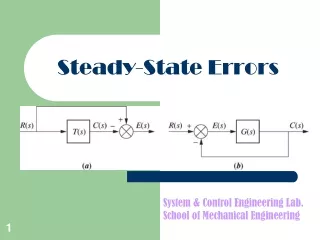
3-5 steady-state error calculation. The steady-state performance is an important characteristic of control system , it represses the ability to follow input signal and resist interference 。 一 .error and steady-state error 1.definition: (1) according to output

E N D
3-5 steady-state error calculation The steady-state performance is an important characteristic of control system , it represses the ability to follow input signal and resist interference。 一.error and steady-state error 1.definition: (1) according to output e(t): system error,Cr(t): requested output, c(t) :practical output。
- Steady-state error: The steady-state error relies on the system's construction ,still the form of the input signal.But stability depends only on system’s construction.
- • (2) according to input
2.calculation (1).final theorem when input is , final theorem can be used.but when input is sine or cosine signal,cannot used. (2).from the definition a.solve error TF
R(s) E(s) + N(s) + b.solve c. solve d. Solve limit that is steady-state error. If the system exists at the same time input and interference,method is as follows:
TF between error and input, TF between error and interference。 so:
n(t)=-1(t) E(s) r(t)=t C(s) - 2 exam:given a block diag. As follows.when input r(t)=t and interference n(t)=-1(t),ess=?
N(s) E(s) C(s) R(s) G1(s) G2(s) - H(s) to interference N(s),we hope it produce output 0,that is ,output is independent of the interference N(s) 。 when input and interference acts on a system,output is respectively:
in this exam.,stability must be assured first,or else,steady-state error cannot exist. 。 Characteristic is:
That is System is stable。 from:
The steady-state error relies on the system's construction ,still the form of the input signal.
二. steady-state error analysis when input acts on a system ---open-loop TF
whenγ=0,1,2 called respectively 0 type system,Ⅰtype system,Ⅱ type system (in generalγ<2) so
Define kp,kv,ka error coefficient。 Step input ,represented by kp position error coefficient。 Speed input, represented by kv velocity error coefficient。 Acceleration input, represented by ka Acceleration error coefficient。
- to increase system type and open-loop gain can increase system's accuracy, but would lower stability, and must consider completely. exam.: given a system.its block diag. is when H(s)=1and H(s)=0.5,solve ess。
When H(s)=1,open-loop TF When H(s)=0.5,
if in exam. above, H(s)=1,ess=0.2,solve k=? when , solve ess in exam. above. Because 0 type system ess = ∞ under the speed input and acceleration input, from addition rule,ess=∞
三.steady state error analysis under interference We hope ess=0 under interference,but it is impossible。 if input R(s)=0, under interference N(s), ess :
E(s) N(s) C(s) R(s) G1(s) G2(s) - H(s)
r(t)=0 C(t) - (a) under interference N(s),steady state output changes, it is connected with open-loop TF G(s)=G1(s)G2(s)H(s) ,interference N(s) and its action position.
r(t)=0 C(t) - (b)
r(t)=0 C(t) - (b) The action position is different, the steady state error is different too. in front of action position,if increase an integer( proportion) to replace
improving integer No.in front of interference action point can decrease or cancel steady state error under interference , but lower the system's stability.
in a word, to decrease steady state error under input, we can increase open-loop TF integer No. and gain. in order to decrease interference error,we must improve integer No.and gain in front of interference action point.this can lower the system's stability,and even transient response goes bad. Following is a good method.
N(s) Gn(s) + C(s) R(s) E(s) G1(s) G2(s) - 四. method of decreasing or canceling steady state error 1. compensation according to interference If interference can be measured ,at the same time,the influence to system is clear and definite, compensation can then improve the steady state accuracy.
Under interference,output: completely cancel the influence to system output. adding compensating equips makes the system's steady state output independent of interference, that is to say, steady state error 0.
Compensation equip. N(s) C(s) R(s)=0 - amplifier filter Exam.: System output:
if selectthe system's output independent of interference,physically too difficult to realize, because the order of denominator of a TF is higher than numerator. if select when steady state, This is completely steady state compensated,and easily realized.
Compensation equipment Gr(s) C(s) G1(s) G2(s) - 2. Compensation according to given input. If completely compensated, R(s)
Similarly, complete compensation is too difficult to realize. usually adopt the steady-state compensation to cancel the steady-state error to some inputs.
No compensation,open-loop TF typeⅠ,input is a ramp,there are some steady-state error.
Introduce compensation Gr(s) to input If select so but is difficult to realize physically。
If take ,so Thus steady-state compensated。
3-8 using Matlab analyze in time domain 3.8.1 stability analysis Pzmap :plot zeros and poles diag. Tf2zp:transform transfer function to zero-pole type Roots:solve roots of a polynominal
>> num=[3 2 5 4 6] num = 3 2 5 4 6 >> den=[1 3 4 2 7 2] den = 1 3 4 2 7 2 >> [z,p,k]=tf2zp(num,den) z = 0.4019 + 1.1965i 0.4019 - 1.1965i -0.7352 + 0.8455i -0.7352 - 0.8455i p = -1.7680 + 1.2673i -1.7680 - 1.2673i 0.4176 + 1.1130i 0.4176 - 1.1130i -0.2991 k = 3 >> pzmap(num,den)
To illustrate the meaning of the following command. roots(den) ans = -1.7680 + 1.2673i -1.7680 - 1.2673i 0.4176 + 1.1130i 0.4176 - 1.1130i -0.2991 >> roots(num) ans = 0.4019 + 1.1965i 0.4019 - 1.1965i -0.7352 + 0.8455i -0.7352 - 0.8455i
3.8.2 transient characteristic analysis Step:solve unit step response num=[25] num = 25 >> den=[1 4 25] den = 1 4 25 >> step(num,den) >> grid
[num,den]=zp2tf([-2],[-1,-0.2+10*i,-0.2-10*i],100) num = 0 0 100 200 den = 1.0000 1.4000 100.4400 100.0400 >> [y,x,t]=step(num,den) subplot(2,1,1),plot(t,y) [yi,xi,t]=impulse(num,den); >> subplot(2,1,2),plot(t,yi)
homework: 3-15 3-18