Download
1 / 38
430 likes | 558 Views
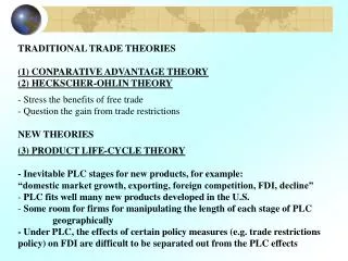
Factor endowments and the Heckscher-Ohlin theory. Dianna DaSilva- Glasgow. outline. Introduction Assumptions of the Model Meaning of the assumptions Factor intensity Factor abundance H-O theory Factor-price equalization and income distribution Leontief Paradox

E N D
Factor endowments and the Heckscher-Ohlin theory Dianna DaSilva- Glasgow
outline • Introduction • Assumptions of the Model • Meaning of the assumptions • Factor intensity • Factor abundance • H-O theory • Factor-price equalization and income distribution • Leontief Paradox • Factor intensity reversal
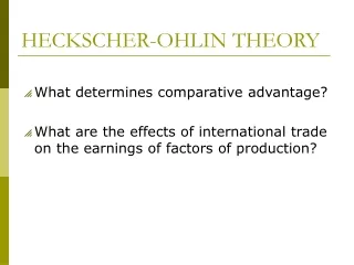
INTRODUCTION • Explain the basis for trade (what determines trade/what determines price differences across countries) • Effect of international trade on the earnings of factors.
ASSUMPTIONS OF THE HO MODEL • Two dimensional model: 2 nations (nation 1 and 2), 2 commodities (X and Y) and 2 factors of production (labour and capital). • Both nations use the same technology in production. • Commodity X is labour intensive and commodity Y is capital intensive in both nations. • Both commodities are produced under constant returns to scale in both nations. • There is incomplete specialization in production in both nations.
ASSUMPTIONS OF THE HO MODEL • Tastes are equal in both nations • There is perfect competition in both commodities and factor markets in both nations. • There is perfect factor mobility within each nation but no international factor mobility • There are no transportation costs, tariffs, or other obstructions to the free flow of international trade • All resources are fully employed in both nations • International trade between the two nations is balanced.
MEANING OF THE ASSUMPTIONS • Assumption 1: Two dimensional model: 2 nations, 2 commodities and 2 factors of production (labour and capital) • Allows for ease of analysis but does not change the theory when relaxed. • Assumption 2: Both nations use the same technology in production • Country’s have access to the same production techniques. With similarity in factor use in the two nations countries will use the cheaper factor more intensively.
MEANING OF THE ASSUMPTIONS • Assumption 3: Commodity X is labour intensive and commodity Y is capital intensive in both nations. • Labor-capital ratio (L/K) is higher for commodity X than Y. • Assumption 4: Both commodities are produced under constant returns to scale in both nations. • Output will increase in the same proportion as the increase in inputs.
MEANING OF THE ASSUMPTIONS • Assumption 5: There is incomplete specialization in production in both nations. • Countries continue to produce both commodities with trade indicating that neither is small. • Assumption 6: Tastes are equal in both nations • Demand preferences; location and shape of the ppf are identical in both nations. Therefore with equal relative commodity prices both nations will consume X and Y in the same proportion.
MEANING OF THE ASSUMPTIONS • Assumption 7: There is perfect competition in both commodities and factor markets in both nations. • Producers of commodities are two small to influence the price of commodities in the commodity market and factors in the factor market. • Assumption 8: There is perfect factor mobility within each nation but no international factor mobility • Factors move freely between industries of low earnings to industries of high earnings until earnings for the same type of factors are the same in all industries.
MEANING OF THE ASSUMPTIONS • Assumption 9: There are no transportation costs, tariffs, or other obstructions to the free flow of international trade • Specialization in production proceeds until relative (and absolute) commodity prices are the same in both nations with trade. • Assumption 10: All resources are fully employed in both nations • There are no unemployed resources in either nation.
MEANING OF THE ASSUMPTIONS • Assumption 11: International trade between the two nations is balanced. • Exports= imports
FACTOR INTENSITY • Measured as: • Relative amount of factor used in the production of commodity. • Example: in nation 1, if 1 capital and 4 labour are used to produce commodity X, then the capital to labour ratio (K/L) = ¼ • In nation 2, if 2 capital and 2 labour are used to produce commodity Y, then K/L = 1 • Therefore: since commodity Y uses more capital per unit of labour than commodity X, commodity Y is the capital intensive commodity, vice versa.
FACTOR INTENSITY • Relative not absolute amounts determine factor intensity • Example: 3K, 12L in the production of commodity X, therefore K/L = 3/12= ¼
FACTOR INTENSITY • On the PPF factor intensity is determined by the slope of the curve. • Commodity Y remains the K-intensive commodity at all possible relative factor prices
Nation 2 Nation 2 has a higher K/L in the production of both commodities reflecting that r/w is lower in nation 2.
FACTOR ABUNDANCE • Factor abundance/endowments refer to the quantity and quality of labor, land, and natural resources of a country.
FACTOR ABUNDANCE • Defined by: • Relative amounts of physical units: nation 2 is capital abundant if the total amount of capital (TK) is greater than the total amount of labour (TL) , (TK/TL)2 > (TK/TL)1 • Relative factor prices: nation 2 is capital abundant if the ratio of the rental price of capital to the price of labour is lower in nation 2, (PK/PL)2 < (PK/PL)1 or (r/w)2 < (r/w)1 • With (TK/TL)2 > (TK/TL)1 then (PK/PL)2 < (PK/PL)1 • The first definition is related only to supply while the latter considers both supply and demand. • Factor endowment seems to explain a significant portion of actual world trade patterns. (Case Study 5.1 and 5.2)
Factor abundance and the ppf The K-abundant nation will export the k-intensive commodity, vice versa
HECKSCHER-OHLIN THEORY • Eli Heckscher, (1919) “The Effect of Foreign Trade on the Distribution of Income” • Bertil Ohlin, (1933) “Interregional and International Trade” • Heckscher- Ohlin Theory: • H-O theorem • Factor-price equalization theorem
THE HECKSCHER-OHLIN THEOREM A nation will export the commodity whose production requires the intensive use of the nation’s relatively abundant and cheap factor and import the commodity whose production requires the intensive use of the nation’s relatively scarce and expensive factor.
THE HECKSCHER-OHLIN THEOREM • Therefore comparative advantage is determined by the difference in relative factor abundance/endowments (factor-endowment theory). • A short list of factors account for a large portion of world trade patterns: natural resources, knowledge capital, physical capital, land, and skilled and unskilled labor.
Illustration of the HO theorem Indifference curve is tangent to both ppfs because of the assumption of same tastes
FACTOR- PRICE EQUALIZATION AND INCOME DISTRIBUTION • Factor price equalization theorem is a corollary of the HO theorem • Paul Samuelson • Heckscher-Ohlin- Samuelson theorem
FACTOR- PRICE EQUALIZATION AND INCOME DISTRIBUTION International trade will bring about equalization in the relative and absolute returns to homogenous factors across nations. • Therefore, international trade is a substitute for the international mobility of factors. • Wages in the low wage country will rise while wages in high wage country will fall until relative wages are equal in the two nations, vice versa.
N1= A where W/R is lower and N2=A’ where W/R is higher. As nation 1 specializes in X and increases demand for labour w/r will rice vice versa Illustration
EFFECT OF TRADE ON THE DISTRIBUTION OF INCOME • Stolper- Samuelson theorem • International trade causes the real income of labour to rise in the labour abundant country and the real income of capital to fall. • Real incomes move with commodity prices with full employment of resources.
SPECIFIC FACTORS MODEL • The distribution of income changes where there are specific factors • The specific-factors model considers the effect of international trade on the distribution of income where there are factors specific to industries. • Example: Commodity X is labour intensive and Commodity Y is capital intensive in Nation 1. However, there is capital specific to each industry. • With trade nation 1 will specialize in commodity X.
SPECIFIC FACTORS MODEL • Nominal wages for workers in industry X increases because of the increase in the relative price of X (Px/Py) • However, the effect of this on the real wage rate is ambiguous because the price increase is greater than the increase in nominal wages leading to a fall in real wages for X and an increase in real wages for Y (price of Y declined)
SPECIFIC FACTORS MODEL • However, with specific factors the effect is clear cut. With trade and the transfer of labour, the real return to capital (used in the production of X) increases as more labour is added to fixed units of capital. • Therefore the model concludes that trade will have an ambiguous effect on the nation’s mobile factors, benefit the immobile factors specific to the nation’s export commodities or sectors, and harm the immobile factors specific to the nation’s import- competing commodities or sectors.
SPECIFIC FACTORS MODEL • However, since the assumptions of the H-O-S theory does not hold in the real world there isn’t evidence of equalization of earnings by homogenous labour across countries.
THE LEONTIEF PARADOX • Wassily Leontief (1951) tested the H-O model empirically, using 1947 US data. He measured the labour and capital content of a representative basket of exports and import-competing goods in the US. • His findings disproved the H-O model as he found that US import substitutes were about 30% more K-intensive than US exports despite the fact that the US is the more K-abundant nation.
THE LEONTIEF PARADOX • Explanations of the paradox: • The year was too close to WWII. The paradox was reduced when a later year 1951 was used • A two- factor model was used • US tariff policy- the most heavily protected industries in the US are L-intensive • Leontief considered only physical capital in his measure of capital ignoring human capital. • The importance of R&D
Factor-intensity reversal • Commodity X is L- intensive in nation 1 (the L-abundant nation) but K-intensive in nation 2 (the K-abundant nation). This would invalidate the HO and factor-price equalization theorem. However, research has found that it rarely occurs. (Study by Minhas in 1962)
Summary • Under the HO model, the difference in factor endowments (in the face of equal technology and tastes) is the basic determinant or cause of comparative advantage.
Further reading • Salvatore (2007) , Chapter 5 • Krugman and Obstfeld (2009), Chapters 1 and 2