Download
1 / 12
130 likes | 161 Views
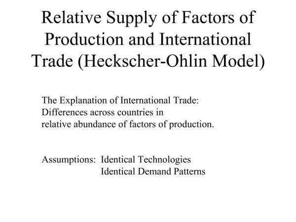
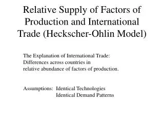
Trade and Resources The Heckscher-Ohlin model. Dr. Petre Badulescu. Introduction. This lecture outlines the Heckscher-Ohlin model , a model that assumes that trade occurs because countries have different resources. Our first goal is to describe the Heckscher-Ohlin (HO) model of trade.

E N D
Trade and ResourcesThe Heckscher-Ohlin model Dr. Petre Badulescu
Introduction This lecture outlines the Heckscher-Ohlin model, a model that assumes that trade occurs because countries have different resources. • Our first goal is to describe the Heckscher-Ohlin (HO) model of trade. • The specific-factors model that we studied in the previous lecture was a short-run model because capital and land could not move between the industries. • In contrast, the HO model is a long-run model because all factors of production can move between the industries. Lecture 4, International economics
Introduction • Our second goal is to examine the empirical evidence on the Heckscher-Ohlin model. • By allowing for more than two factors of production and also allowing countries to differ in their technologies, as in the Ricardo model, the predictions from the Heckscher-Ohlin model match more closely the trade patterns in the world economy today. • The third goal of the lecture is to investigatehow the opening of trade between the two countries affects the payments to labor and to capital in each of them. Lecture 4, International economics
The Heckscher-Ohlin Model Assumptions Assumption 1: Two factors of production, labor (L) and capital (K), can move freely between the industries. Assumption 2: Shoe production is labor-intensive; that is, it requires more labor per unit of capital to produce shoes than computers, so that LS/KS>LC/KC. Lecture 4, International economics
The Heckscher-Ohlin Model Assumptions Labor Intensity of Each Industry The demand for labor relative to capital is assumed to be higher in shoes than in computers, LS/KS> LC/KC. FIGURE 4-1 These two curves slope down just like regular demand curves, but in this case, they are relative demandcurves for labor (i.e., demand for labor divided by demand for capital). 0 Lecture 4, International economics
The Heckscher-Ohlin Model Assumptions Assumption 3: Foreign is labor-abundant, by which we mean that the labor–capital ratio in Foreign exceeds that in Home, L*/K*>L/K. Equivalently, Home is capital-abundant, so that K/L>K*/L*. Assumption 4: The final outputs, shoes and computers, can be traded freely (i.e., without any restrictions) between nations, but labor and capital do not move between countries. Lecture 4, International economics
The Heckscher-Ohlin Model Assumptions Assumption 5: The technologies used to produce the two goods are identical across the countries. Assumption 6: Consumer tastes are the same across countries, and preferences for computers and shoes do not vary with a country’s level of income. Lecture 4, International economics
APPLICATION Are Factor Intensities the Same across Countries? While much of the footwear in the world is produced in developing nations, the United States retains a small number of shoe factories. In India, the sewing machine used to produce footwear is cheaper than the computer used in a call center. Footwear production in India is labor-intensive as compared with the call center, which is the opposite of what holds in the United States. This example illustrates a reversal of factor intensities between the two countries. In the United States, agriculture is capital-intensive. In many developing countries, it is labor-intensive. ■ Lecture 4, International economics
The Heckscher-Ohlin Model No-trade equilibrium PPF:s, Indifference Curves, and No-Trade Equilibrium Price No-Trade Equilibriain Home and Foreign FIGURE 4-2 (1 of 3) 0 0 The Home production possibilities frontier (PPF) is shown in panel (a), and the Foreign PPF is shown in panel (b). Because Home is capital abundant and computers are capital intensive, the Home PPF is skewed toward computers. Lecture 4, International economics
The Heckscher-Ohlin Model No-trade equilibrium PPF:s, Indifference Curves, and No-Trade Equilibrium Price FIGURE 4-2 (2 of 3) No-Trade Equilibriain Home and Foreign (continued) 0 0 Home preferences are summarized by the indifference curve, U. The slope of an indifference curve equals the amount that consumers are willing to pay for computers in terms of shoes rather than dollars. The Home no-trade (or autarky)equilibrium is at the tangency point A, where the relative price that consumers are willing to pay for one more computer equals the opportunity cost of producing it. The flat slope indicates a low relative priceof computers, (PC /PS)A. The slope of the PPF equals the opportunity cost of producing one more computer in terms of shoes given up. Lecture 4, International economics
The Heckscher-Ohlin Model No-trade equilibrium PPF:s, Indifference Curves, and No-Trade Equilibrium Price FIGURE 4-2 (3 of 3) No-Trade Equilibriain Home and Foreign (continued) A* 0 0 Foreign is labor-abundant and shoes are labor- intensive, so the Foreign PPF is skewed toward shoes. Foreign preferences are summarized by the indifference curve, U* The Foreignno-trade equilibrium is at the tangency point A*, with a higher relative price of computers, as indicated by the steeper slope of (P*C /P*S)A*. The result from comparing the no-trade equilibria for these two countries is that the no-trade relative price of computers at Home is lower than in Foreign. Lecture 4, International economics
The Heckscher-Ohlin Model Free-trade equilibrium We are now in a position to determine the pattern of trade between the two countries. We proceed in several steps. First, we consider what happens when the world relative price of computers is above the no-trade relative price of computers at Home, and trace out the Home export supply of computers. Second, we consider what happens when the world relative price is below the no-trade relative price of computers in Foreign, and trace out the Foreign import demand for computers. Finally, we put together the Home export supply (Sx) and the Foreign import demand (Dm) to determinethe equilibrium relative market price of computers with international trade. Ch 041.pptx Lecture 4, International economics