Download
1 / 22
240 likes | 360 Views
Register Allocation. Harry Xu CS 142 (b) 02/11/2013. Register Allocation. Assigning a large number of program variables to a small number of CPU registers for improved performance Motivation A developer often allocates arbitrarily many variables

E N D
Register Allocation Harry Xu CS 142 (b) 02/11/2013
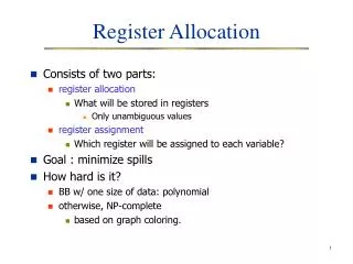
Register Allocation • Assigning a large number of program variables to a small number of CPU registers for improved performance • Motivation • A developer often allocates arbitrarily many variables • The compiler must decide how to allocate these variables to a small, finite set of registers
Basic Idea • Variable liveness analysis • Two variables that will be used at the same time cannot be allocated to the same register • Some variables will be held in RAM and loaded in/out for every read/write, a process called spilling • Assigning as many variables to registers as possible • Memory accesses are slower
Reaching Definition Analysis • A classic dataflow analysis to understand what variables are live simultaneously at a given program point • A backward analysis that computes dataflow facts from the end of the program • Given an (SSA) statement s, there are four important sets the analysis needs to maintain • Gen[s]: the set of variables used in s • Kill[s]: the set of variables that are assigned values in s • Live-in[s]: the set of variables that are simultaneously live before s is executed • Live-out[s]: the set of variables that are simultaneously live after s is executed
Liveness Analysis (Cond) • Initial setup • Live-out[final] = ∅ • Gen[a:= b + c] = {b, c} • Kill[a:= b + c] = {a} • Dataflow equations • Lives-in[s] = Gen[s] ∪(Lives-out[s] – Kill[s]) • Lives-out[s] = ∪p∊succ(s)Live-in[p]
An Example Gen(L1) = {}, Kill(L1) = {a} Gen(L2) = {}, Kill(L2) = {b} Gen(L3) = {}, Kill(L3) = {d} Gen(L4) = {}, Kill(L4) = {x} Gen(L5) = {a, b}, Kill(L5) = {} Gen(L6) = {a, b}, Kill(L6) = {c} Gen(L7) = {}, Kill(L7) = {d} Gen(L8) = {}, Kill(L8) = {} Gen(L9) = {}, Kill(L9) = {c} Gen(L10) = {b, d, c}, Kill(L5) = {} L1: a = 3; L2: b = 5; L3: d = 4; L4: x = 100; L5: if a > b then L6: c = a + b; L7: d = 2; L8: endif L9: c = 4; L10:return b * d + c; • Worklist = { L10 }
Compute Liveness L1: a = 3; L2: b = 5; L3: d = 4; L4: x = 100; L5: if a > b then L6: c = a + b; L7: d = 2; L8: endif L9: c = 4; L10:return b * d + c; Live-out = {} Live-in = {b, d, c} • Lives-in[s] = Gen[s] ∪(Lives-out[s] – Kill[s]) • Lives-out[s] = ∪p∊succ(s)Live-in[p] • Worklist = {L9}
Compute Liveness L1: a = 3; L2: b = 5; L3: d = 4; L4: x = 100; L5: if a > b then L6: c = a + b; L7: d = 2; L8: endif L9: c = 4; L10:return b * d + c; Live-out = {b, d, c} Live-in = {b, d} Live-out = {} Live-in = {b, d, c} • Lives-in[s] = Gen[s] ∪(Lives-out[s] – Kill[s]) • Lives-out[s] = ∪p∊succ(s)Live-in[p] • Worklist = {L8}
Compute Liveness L1: a = 3; L2: b = 5; L3: d = 4; L4: x = 100; L5: if a > b then L6: c = a + b; L7: d = 2; L8: endif L9: c = 4; L10:return b * d + c; Live-out = {b,d} Live-in = {b, d} Live-out = {b,d,c} Live-in = {b, d} Live-out = {} Live-in = {b, d, c} • Lives-in[s] = Gen[s] ∪(Lives-out[s] – Kill[s]) • Lives-out[s] = ∪p∊succ(s)Live-in[p] • Worklist = {L7, L5}
Compute Liveness L1: a = 3; L2: b = 5; L3: d = 4; L4: x = 100; L5: if a > b then L6: c = a + b; L7: d = 2; L8: endif L9: c = 4; L10:return b * d + c; Live-out = {b, d} Live-in = {b} Live-out = {b,d} Live-in = {b, d} Live-out = {b, d, c} Live-in = {b, d} Live-out = {} Live-in = {b, d, c} • Lives-in[s] = Gen[s] ∪(Lives-out[s] – Kill[s]) • Lives-out[s] = ∪p∊succ(s)Live-in[p] • Worklist = {L6, L5}
Compute Liveness L1: a = 3; L2: b = 5; L3: d = 4; L4: x = 100; L5: if a > b then L6: c = a + b; L7: d = 2; L8: endif L9: c = 4; L10:return b * d + c; Live-out = {b} Live-in = {b, a} Live-out = {b, d} Live-in = {b} Live-out = {b, d} Live-in = {b, d} Live-out = {b, d, c} Live-in = {b, d} Live-out = {} Live-in = {b, d, c} • Lives-in[s] = Gen[s] ∪(Lives-out[s] – Kill[s]) • Lives-out[s] = ∪p∊succ(s)Live-in[p] • Worklist = {L5}
Compute Liveness L1: a = 3; L2: b = 5; L3: d = 4; L4: x = 100; L5: if a > b then L6: c = a + b; L7: d = 2; L8: endif L9: c = 4; L10:return b * d + c; Live-out = {b, a, d} Live-in = {b, a, d} Live-out = {b} Live-in = {b, a} Live-out = {b, d} Live-in = {b} Live-out = {b, d} Live-in = {b, d} Live-out = {b, d, c} Live-in = {b, d} Live-out = {} Live-in = {b, d, c} • Lives-in[s] = Gen[s] ∪(Lives-out[s] – Kill[s]) • Lives-out[s] = ∪p∊succ(s)Live-in[p] • Worklist = {L4}
Compute Liveness L1: a = 3; L2: b = 5; L3: d = 4; L4: x = 100; L5: if a > b then L6: c = a + b; L7: d = 2; L8: endif L9: c = 4; L10:return b * d + c; Live-out = {b, a, d} Live-in = {b, a, d} Live-out = {b, a, d} Live-in = {b, a, d} Live-out = {b} Live-in = {b, a} Live-out = {b, d} Live-in = {b} Live-out = {b, d} Live-in = {b, d} Live-out = {b, d, c} Live-in = {b, d} Live-out = {} Live-in = {b, d, c} • Lives-in[s] = Gen[s] ∪(Lives-out[s] – Kill[s]) • Lives-out[s] = ∪p∊succ(s)Live-in[p] • Worklist = {L3}
Compute Liveness L1: a = 3; L2: b = 5; L3: d = 4; L4: x = 100; L5: if a > b then L6: c = a + b; L7: d = 2; L8: endif L9: c = 4; L10:return b * d + c; Live-out = {b, a, d} Live-in = {b, a} Live-out = {b, a, d} Live-in = {b, a, d} Live-out = {b, a, d} Live-in = {b, a, d} Live-out = {b} Live-in = {b, a} Live-out = {b, d} Live-in = {b} Live-out = {b, d} Live-in = {b, d} Live-out = {b, d, c} Live-in = {b, d} Live-out = {} Live-in = {b, d, c} • Lives-in[s] = Gen[s] ∪(Lives-out[s] – Kill[s]) • Lives-out[s] = ∪p∊succ(s)Live-in[p] • Worklist = {L2}
Compute Liveness L1: a = 3; L2: b = 5; L3: d = 4; L4: x = 100; L5: if a > b then L6: c = a + b; L7: d = 2; L8: endif L9: c = 4; L10:return b * d + c; Live-out = {b, a} Live-in = {a} Live-out = {b, a, d} Live-in = {b, a} Live-out = {b, a, d} Live-in = {b, a, d} Live-out = {b, a, d} Live-in = {b, a, d} Live-out = {b} Live-in = {b, a} Live-out = {b, d} Live-in = {b} Live-out = {b, d} Live-in = {b, d} Live-out = {b, d, c} Live-in = {b, d} Live-out = {} Live-in = {b, d, c} • Lives-in[s] = Gen[s] ∪(Lives-out[s] – Kill[s]) • Lives-out[s] = ∪p∊succ(s)Live-in[p] • Worklist = {L1}
Compute Liveness L1: a = 3; L2: b = 5; L3: d = 4; L4: x = 100; L5: if a > b then L6: c = a + b; L7: d = 2; L8: endif L9: c = 4; L10:return b * d + c; Live-out = {a} Live-in = { } Live-out = {b, a} Live-in = {a} Live-out = {b, a, d} Live-in = {b, a} Live-out = {b, a, d} Live-in = {b, a, d} Live-out = {b, a, d} Live-in = {b, a, d} Live-out = {b} Live-in = {b, a} Live-out = {b, d} Live-in = {b} Live-out = {b, d} Live-in = {b, d} Live-out = {b, d, c} Live-in = {b, d} Live-out = {} Live-in = {b, d, c} • Lives-in[s] = Gen[s] ∪(Lives-out[s] – Kill[s]) • Lives-out[s] = ∪p∊succ(s)Live-in[p] • Worklist = {}
Handling of Loops • A fixed-point computation needs to be performed • The next statement is not added into the worklist if Live-out and Live-in of the current statement no longer change
Interference Graph • Each node represents a variable • Each edge connects two variables which can be live at the same time • Register allocation is reducedto the problem of k-coloring the interference graph a b x c d
K-Coloring • An NP-complete problem • For this graph, three colors are sufficient a b x c d
Algorithms • Brute-force search • Try every of the kn assignments of k colors to n vertices and checks if each assignment is legal • The process repeats for k = 1, 2, …, n – 1 • Impractical for all but small input graphs • Other algorithms • Dynamic programming • Parallel algorithms
X86 Registers • General registers • EAX EBX ECX EDX • Segment registers • CS DS ES FS GS SS • Index and pointers • ESI EDI EBP EIP ESP • Indicator EFLAGS • Never use EBX and EBP
Output • For each register, the set of variables that can be allocated to it • The result of this phase will be used by the final code generation phase to guide the actual register allocation