Download
1 / 34
340 likes | 551 Views
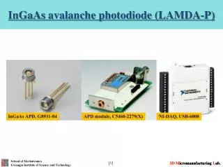
Computing Bit-Error Probability for Avalanche Photodiode Receivers by Large Deviations Theory. Abhik Kumar Das Indian Institute of Technology, Kanpur under the guidance of Majeed M. Hayat and P. Sun UNM, Albuquerque. OUTLINE. APD: Introduction APD: Gain and Build-up Time Relation

E N D
Computing Bit-Error Probability for Avalanche Photodiode Receivers by Large Deviations Theory Abhik Kumar Das Indian Institute of Technology, Kanpur under the guidance of Majeed M. Hayat and P. Sun UNM, Albuquerque
OUTLINE • APD: Introduction • APD: Gain and Build-up Time Relation • Joint PDF of Gain & Build-up Time – Renewal Relations • Numerical Computation • Large Deviations Theory • Cramér's Theorem • Gärtner-Ellis Theorem
APD: Bit-ErrorProbability Computation • Literature Review • Sadowsky and Letaief • Hayat and B. Choi • Generalized Theory • Bit-Error Probability Estimation • Large Deviations/Asymptotic Analysis • Gaussian Approximation • Numerical Results • Conclusion
APD : Introduction • APD - • used in high-speed optical receivers • offers high opto-electronic gain • Functioning - • photon-impacts produce primary carriers • primary carriers move due to electric field to produce secondary carriers by avalanche process in multiplication layer • these carriers constitute the photo-current • Impulse-response of APD stochastic in nature with both random gain and impulse duration/build-up time
Multiplication Layer First impact ionization Injected electron • Avalanche Process - p n de de dh dh de x W Eieand Eih are the average ionization threshold energies Hole Electron Dead space for electron Dead space for hole Electric field E
Gain and Build-up Time Relation • Joint PDF of gain G and build-up time T - • defined as m = no. of electron-hole pairs produced t = time before completion of avalanche build-up • Hayat and P. Sun proposed a method to compute it from coupled renewal relations mentioned below -
parent electron first impact ionization p n x + x 0 W • Physical Interpretation of Renewal Relations - • andare the intermediate quantities and +V
Recursive Equations for some fixed z, and suitable range of t & x Recursive Equations z-transform over m Compute relative change Update data No Initialize data If <tolerance level Gubner and Hayat method Final result (for fixed z and hence m) Yes • Numerical Computation -
Joint distribution function (PDF) of G and T for homo-junction GaAs APD with 160 nm – multiplication layer and average gain 10.46 Joint density function of G and T for the same APD. Large peaks have been truncated to show details
Large Deviations Theory • Theory of ‘rare’ events - • concerned with the behavior of ‘tails’ of probability distributions • Law of Large Numbers – special case of the theory • Cramér's Theorem - • concerned with i.i.d. random variable sequence • most basic theorem of the theory • Gärtner-Ellis Theorem - • generalizes Cramér's Theorem • can be applied to independent, but not necessarily identical random variable sequence
Corollary of Cramér's Theorem - Deduction from Corollary -
Bit-Error Probability Computation Literature Review • Sadowsky and Letaief - • gave an asymptotic analysis method based on large deviations theory for error probability estimation • formulated an efficient Monte-Carlo estimation method based on importance sampling • assumptions made in the theory: • dead-space effect neglected • APD functioning considered to be instantaneous • OOK-type modulated optical signal • direct detection integrate-and-dump receiver
Salient Points of the Theory – • Define • Gk = gain of kth primary electron • M = no. of primary electrons in signaling interval • N = thermal noise response of receiver with variance σ2 • Assume {Gk} to be i.i.d. This gives the receiver statistic as: • Consider the hypotheses: • Let γ be the decision threshold, define:
Bit-error probability is given as: • Asymptotic Analysis – • Define , , The function is steep if . • The mgf for G given by McIntyre was used by Sadowsky and Letaief, which doesn’t include dead-space effect. • Let γ = (1/c0)λ0 = (1/c1)λ1, c0 and c1 positive constants. Asymptotic refers to γ being large. • The estimate for bit-error probability can be obtained from a result proven by Sadowsky and Letaief.
Monte-Carlo Estimation – • A sequence D(l) = (M(l),G(l),N(l)), l = 1,2,…,L, is generated according to their twisted distributions. • The error probability is estimated using: where 11(D) = 1 if D< γ, zero otherwise; and 10(D) = 1 if D> γ, zero otherwise. • W(•) is the importance-sampling weighting function, it was chosen as:
Hayat and B. Choi – • modified the work of Sadowsky and Letaief to include dead-space effect • other assumptions were held intact • same approach was adopted, only dead-space generalized mgf for G was used in place of the one given by McIntyre • similar approach was also used for Monte-Carlo estimation
Generalized Theory • The generalized theory, takes into account dead-space effect and doesn’t assume instantaneous functioning of APD. • The theory uses the model for APD as proposed by Hayat; impulse-response of APD is considered to be a random-duration rectangular function. • Salient points of the Theory- • Consider the time interval [0,Tb] and assume current information bit as ‘1’. Let Gi, Ti be gain and impulse-response duration due to ith primary electron and τi be the time of impact. Let indicator function for set A be defined as 1A(x) = 1, x an element of A, zero otherwise. Defining , gives photocurrent as In case of bit ‘0’, it is assumed Gi = 0 for all i.
The photocurrent functioncan be approximated by dividing [0,Tb] into N equal slots and assuming in each slot all photons get absorbed at same time t = τi = i(Tb/N). Let ni be no. of absorptions in ith slot, Gij and Tij be gain and duration for jth absorption in ith slot, then • The receiver’s output at index ‘k’ is then • We define to get
We examine R0 and evaluate mgf of A0,j(τi) as • I is a boolean function function with I(x) = 1, if x is true, zero otherwise. Total no. of photons is a Poisson variable with parameter, say λ, then ni can be assumed to be a Poisson variable with parameter (λ/N), so that mgf of R0 can be found out as:
Likewise, mgf of Rk, Rk(μ) can be found as • With respect to [0,Tb], R0 conveys information about current bit, R1 conveys information about previous bit, in general, Rk conveys information about kth previous bit, provided the bit-stream entirely consists of ‘1’s. For general bit-stream, the receiver output is:
Bit-Error Probability Estimation • For the sake of simplicity, we consider R0, R1, R2 only so that receiver output Yλ becomes: • Decision threshold γ is defined as: which simplifies to
Bit-error probability is then given by: • Means and variances for Yλ when current bit is ‘1’ and ‘0’ are:
The following relations help in calculating the means and variances:
Large Deviations Theory • {Yλ} can be seen as an infinite sequence of random variables w.r.t. λ. We define which on simplification gives • Defining corresponding to cases of current bit being ‘0’ and ‘1’ gives
where (•)+ is a function defined as (x)+ = x, x>0, zero else. • The rate functions I0(x) and I1(x) can be computed as: • Assuming Hypothesis 1 of Gärtner-Ellis Theorem is true, we have
Letting and gives • This gives an approximate expression for bit-error probability:
Gaussian Approximation • For Gaussian approximation, we assume Yλ ~ N(ρ0,σ02) when current bit is ‘0’ and Yλ ~ N(ρ1,σ12) when current bit is ‘1’. • Then, bit-error probability is given as:
Numerical Results • Computation of bit-error probability was carried out for InP APD receiver with 100-nm multiplication layer and average gain 10.699. • The optical-link speed was 40 Gbps (i.e. 1/Tb = 40 Gbps), the time interval was divided into N = 1000 equal slots and value of decision threshold was γ = 5.325. • A plot for λ (average no. of photons in the time interval) vs. bit-error probability was made, with λ ranging from 1000 to 3000.
Conclusion • The generalized theory – • takes into account dead space effect • assumes the functioning of APD to be non-instantaneous • The use of asymptotic-analysis techniques and other approximation methods are extended to a wider class of APDs. • Large Deviations give a better estimate of error probability compared to Gaussian approximation.