Download
1 / 19
190 likes | 322 Views
Finding a Given Proportion, Assessing Normality 2.2c. Target Goal: I can find the raw value of a score given a z score. I can determine the normality of a given set of data. h.w : pg 133: 63, 65, 66, 68 -74. Normal Distributions.

E N D
Finding a Given Proportion, Assessing Normality2.2c Target Goal: I can find the raw value of a score given a z score. I can determine the normality of a given set of data. h.w: pg 133: 63, 65, 66, 68 -74
Normal Distributions • The normal distribution is an easy to use approximation, not a description of every detail in the actual data. • x > 240 vs x ≥ 240: There is no area under the curve and exactly over 240, so the area x > 240 vs x ≥ 240 are the same.
Finding a Value of a Given Proportion To find the observed value with a given proportion above or below it, use Table A and work backward. • “unstandardize” Step 1: State the problem and draw a sketch. Step 2: Plan - Use the table. Step 3: Do - Unstandardize to transform the solution from the z back to the original x scale.
Ex. 1 SAT Verbal Scores Scores on the SAT verbal test follow approximately the N(505,110) distribution. How high must a student score in order to place in the top 10% of all students taking the SAT?
Step 1: State the problem and draw a sketch. Step 1: We want to find the SAT score x with area 0.1 to its right under the normal curve with μ = 505 and σ = 110. (Same as finding the SAT score x with to its left. .90
Step 2: Plan - Use the table. • Look in Table A for the entry closest to 0.9. It is which corresponds to z = 1.28. • Step 3: Do - Unstandardize to transform the solution from the z back to the original x scale. 1.28 = x = 646 0.8997
Ex. 2: Heights of American Men The distribution of adult American men is approximately normal with mean 69 inches and standard deviation 2.5 inches. c. How tall must a man be to be in the tallest 15% of all men?
Step 1: State the problem and draw a sketch. We want to find the z score with area 0.15 to its rightunder the normal curve with μ = 69 and σ = 2.5. Sketch Z= x=69 71.5
Step 2: Plan - Use the table Since we want the area 0.15 to its right, look in Table A for the entry closest to 0.85. It is which corresponds to 0.8485 z = 1.03
Step 3: D0 - Unstandardize • Transform the solution from the z back to the original x scale. ( x - μ ) = z σ (x - 69) = 1.03 2.5 x = 71.575
Exercise 3: Quartiles The quartiles of any density curve are the points with area 0.25 and 0.75to their left under the curve. • What are the quartiles of the standard normal curve? • Look up 0.25 in Table A • 0.25 is between • Look up 0.75 • + 0.675 z = -0.67 and z = -0.68
Standard deviations away from the mean ? b. How many standard deviations away from the mean do the quartiles lie in any normal distribution? • For any normal distribution, the quartiles are 0.675 standard deviations from the mean.
Assessing Normality Method 1: • Construct a frequency histogram or a stemplot. • See if the graph is approx. bell-shaped and symmetric about the mean. • Mark the points; (use sx on calculator). • Compare counts in the interval with empirical rule (68-95-99.7).
Ex 4: Assessing NormalityCompare counts in interval with empirical rule (68-95-99.7). • 649/947 = 68.5% of the data fall within 1 standard deviation of the mean. • Calculate the other intervals.
x bar 2s = • x bar 3s = • The counts confirm that the normal distribution fits the data well. .9535 .9979
Assessing Normality Method 2: Construct a normal probability plot. (see page 128) • Enter data into L1, graph histogram. • Ask for 1-VAR STATS:L1 and compare the means and medians to confirm that the distribution is roughly symmetric.
Method 2 cont. • Construct normal probability plot of the data. {STATPLOT} • Use ZoomStat to see finished graph. • If the data distribution is close to normal, the plotted points will lie close to a straight line.
The data for the survival of 72 guinea pigs in days who were injected with infectious material in a medical experiment were graphed. Pg. 127