Download
1 / 35
390 likes | 582 Views
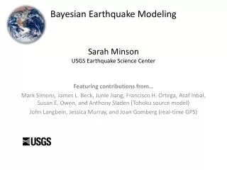
Featuring contributions from… Mark Simons James L. Beck Junle Jiang Francisco H. Ortega Asaf Inbal Susan E. Owen Anthony Sladen. Bayesian Kinematic Earthquake Models Sarah Minson USGS Seattle. Embrace Uncertainty.

E N D
Featuring contributions from… Mark Simons James L. Beck Junle Jiang Francisco H. Ortega AsafInbal Susan E. Owen Anthony Sladen Bayesian Kinematic Earthquake ModelsSarah MinsonUSGS Seattle
Embrace Uncertainty • One of the geophysical community’s failures before the Tohoku earthquake was not emphasizing what we don’t know. • To whatever extent the Tohoku earthquake was unexpected, it was because the uncertainties of the rupture history and plate coupling were not understood • To avoid falling into this trap, we adopt a Bayesian approach to kinematic rupture modeling
Bayes’ Theorem (1763) • For inverse problems: Posterior Prior Data Likelihood
Why not choose Bayesian analysis? • Huge numbers of samples required for high-dimensional problems • “Curse of Dimensionality” • Requires evaluation of billions of forward models • NASA Pleiades supercomputer
Cascading Adaptive Transitional Metropolis In Parallel: CATMIP • Transitioning AKA Tempering AKA Simulated Annealing* • Dynamic cooling schedule** • Parallel Metropolis • Simulation adapts to model covariance** • Simulation adapts to rejection rate*** • Resampling** • Cascading Static Kinematic * Marinari and Parisi (1992) ** Ching and Chen (2007) *** Matt Muto
Example: Mixture of Gaussians • Target distribution:
CATMIP • Sample P(θ) • Calculate β • Resample • Metropolis algorithm in parallel • Collect final samples • Go back to Step 2, lather, rinse, and repeat until cooling is achieved
Model Prediction Errors • Assumed errors control posterior model errors • For geophysical data, εD is often small • Seismograms are accurate, InSAR phases are accurate • For slip models, errors on εG(θ)can be large • Percent error on Gscales with source • Seismograms have background noise, InSAR has atmospheric blobs • These “data errors” represent unmodeled signals • If ε=εDis assumed, total error is under-estimated
Posterior mean with model prediction error is not better than mean without prediction error • Bad model = can’t recover true solution • But the posterior 95% confidence with prediction error more accurately represents the real uncertainty
A Bayesian Exploration of Kinematic Rupture Parameters for the Great 2011 Tohoku-Oki Earthquake
Methodology • Choose a finite discretized planar fault model (strike constant, dip increasing from 3°-29°), hypocenter and elastic structure • This is our model design • Broad priors • Use Bayesian inference to determine posterior PDFs of slip distributions which fit available static data (GPS, DART, seafloor pressure gauges, seafloor geodesy) • Use posterior PDF as prior for joint static-kinematic source rupture model using 1 Hz GPS • 1-D Green’s functions • STF is triangle • Each patch can only rupture once • Rupture is causal (calculated via Fast Sweeping algorithm) • Assume:
Posterior mean (one statistic of many)Slip duration Rupture velocity
Consistent with previously published preliminary solution Kinematic solution Simons et al. (Science, 2011)
All models Slip is less well constrained as rupture evolves But total moment magnitude is well constrained
One sigma Slip is less well constrained as rupture evolves But total moment magnitude is well constrained
Posterior moment rate Lay and Kanamori (2011)
Along-strike integrated slip • We fit both GPS, seafloor observations, and both near-field and far-field tsunami observations • Both our preliminary model and this model find significant near-trench fault slip but, on average, peak slip is not at the trench • This decrease in slip amplitude near trench is recoverable because the model is not regularized • However, localized zones of high slip may exist near trench
Conclusions • Fully Bayesian kinematic rupture model for the Tohoku-Oki earthquake • Fast preliminary slip model is consistent with full kinematic solution • Significant slip near trench, but peak large-scale slip feature is not at trench • A wide range of data are very well-fit • Model prediction error is essential to estimating uncertainty in solution • Uncertainty in slip model is essential to understanding the subduction zone
Earthquake monitoring using GPS • Dense real-time 1 Hz GPS network • Utilize GPS with seismic data to identify and analyze events for which GPS data contribute the most • Hazardous earthquakes • Slow slip events
Rapid response vs. early warning • Rapid response • Real-time event detection • On-demand source analysis • Real-time Bayesian magnitude determination for EEW • Proper alarm criterion is “Mw > threshold with x% confidence”