Download
1 / 43
510 likes | 787 Views
Computer Graphics Lecture 10 Global Illumination 1: Ray Tracing and Radiosity. Taku Komura. Rendering techniques. Can be classified as Local Illumination techniques Global Illumination techniques. Local Illumination methods . Considers light sources and surface properties only.

E N D
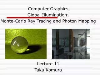
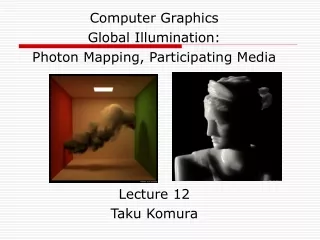
Computer GraphicsLecture 10Global Illumination 1: Ray Tracing and Radiosity Taku Komura
Rendering techniques • Can be classified as • Local Illumination techniques • Global Illumination techniques
Local Illumination methods • Considers light sources and surface properties only. • Phong Illumination, Phong shading, Gouraud Shading • Using techniques like Shadow maps, shadow volume, shadow texture for producing shadows • Very fast • Used for real-time applications such as 3D computer games
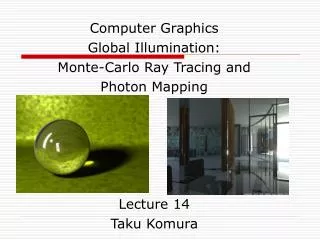
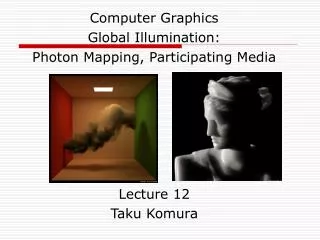
Global Illumination • Methods that simulate not only the direct illuminations but also the indirect illuminations • Monte-Carlo ray tracing • Radiosity, Photon Mapping • Global illuminations can handle • Reflection (one object in another) • Refraction (Snell’s Law) • Shadows • Colour bleeding under the same framework • Requires more computation and is slow
Today : Global Illumination Modules and Methods • Ray Tracing • Radiosity
Ray Tracing [Appel ’68] • Ray tracing is one of the most popular methods used in 3D computer graphics to render an image • Good at simulating specular effects • Tracing the path taken by a ray of light through the scene • Rays are reflected, refracted, or absorbed whenever intersect an object • Can produce shadows
Shadow • If the ray hits an object, we want to know if that point on the object is in a shadow. • So, when the ray hits an object, a secondary ray, called a "shadow" ray, is shot towards the light sources
Shadow(2) • If this shadow ray hits another object before it hits a light source, then the first intersection point is in the shadow of the second object. • We only apply the ambient term for that light source. • Otherwise do the local Phong Illumination and expand the Ray Tree
Shadow (3) • First Intersection point in the shadow of the second object
Reflected Ray • Also, when a ray hits an object, a reflected ray is generated which is tested against all of the objects in the scene.
Contribution from the reflected ray • If the reflected ray hits an object then a local illumination model is applied at the point of intersection and the result is carried back to the first intersection point.
Transmitted Ray • If the intersected object is transparent, then a transmitted ray is generated and tested against all the objects in the scene
Contribution from the transmitted ray • As with the reflected ray, if the transmitted ray hits an object then a local illumination model is applied at the point of intersection and the result is carried back to the first intersection point.
Ray Tree [Whitted ‘80] • Fire off secondary rays from surface that ray intersects. • Towards Light Source(s) : shadow rays. L (shadow feelers) • In the reflection direction : reflection rays, R • In a direction dictated by Snell’s Law : transmitted rays, T
Recursive ray tree. • Reflection and Transmission Rays spawn other rays. • Shadow rays used to check occlusion / local illumination of diffuse surfaces • Brightness recursively computed by I = Ilocal + Kr * R + Kt * T where Ilocal is the color by local illumination, R is the color by reflection, T is the color by transmission, and Kr, Kt are coefficients • The complete set of rays is called a Ray Tree. Light Source ray determines colour of current object. Viewpoint
Test Scene. Ray tree depth 1. Note only ambient shade on mirror and teapot
Test Scene. Ray tree depth 2. Note only ambient shade on reflection of mirror and teapot.
Test Scene. Ray tree depth 3. Note only ambient shade on reflection of mirror in teapot.
Test Scene. Ray tree depth 4. Note ambient shade on reflection of teapot in reflection of mirror in teapot.
Test Scene. Ray tree depth 5.
Test Scene. Ray tree depth 6.
Test Scene. Ray tree depth 7.
When to stop ? • When the a ray hits a perfectly diffusive surface • For specular surface, we can define a fixed depth
Adaptive tree depth control. • Calculate maximum contribution of a ray to a pixels final value. • For example, if the surface is more diffusive, smaller influence from the reflection ray • Multiply contribution of ray’s ancestors down the tree. • Stop when below some threshold • In the case above, stop when Hall, R. A. and Greenberg D.P. , "A Testbed for Realistic Image Synthesis", IEEE Computer Graphics and Applications, 3(8), Nov., 1983
Ray-polygon intersection. • Not so easy ! • Determine whether ray intersects polygon’s plane. • Determine whether intersection lies within polygon. • Easiest to determine (2) with an orthographic projection onto the nearest axis and the 2D point-in-polygon test. • Then calculate the barycentric coordinates http://www-graphics.stanford.edu/courses/cs348b-98/gg/intersect.html z Ray x y
Accelerating Ray Tracers • Ray Tracing is very time-consuming because of intersection calculations • Solutions: • Use faster machines • Use specialized hardware, especially parallel processors. • Use perspective projection for the first ray • Use a larger threshold for adaptive depth tree control • Reduce the number of rays / polygon intersection check • Bounding volumes
Reducing Ray-Object Intersections • Bounding Volumes: • Enclose groups of objects in sets of hierarchical bounding volumes • Octree • First test for intersection with the bounding volume • Then only if there is an intersection, against the objects enclosed by the volume.
Ray Tracing : Drawbacks • Can we produce soft shadows? • Can we produce bleeding effects? • Can we render caustics? • Can we generate shadows of refractive objects?
Tough Cases • Caustics • Light focuses through a specular surface onto a diffuse surface • Which direction should secondary rays be cast to detect caustic? • Bleeding • Color of diffuse surface reflected in another diffuse surface • Which direction should secondary rays be cast to detect bleeding? Tracking the light source after hitting diffuse surface is not very easy
Today : Global Illumination Modules and Methods • Ray Tracing • Radiosity
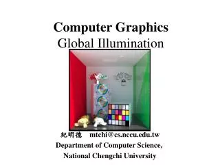
The Radiosity Method (84’-) • Can produce soft shadows, colour bleeding • View independent the rendering calculation does not have to be done although the viewpoint is changed • The basic method can only handle diffuse color → need to be combined with ray-tracing to handle specular light
The Radiosity Model • At each surface in a model the amount of energy that is given off (Radiosity) is comprised of • the energy that the surface emits internally (E), plus • the amount of energy that is reflected off the surface (ρH)
The Radiosity Model(2) • The amount of incident light hitting the surface can be found by summing for all other surfaces the amount of energy that they contribute to this surface
Form Factor (Fij) • the fraction of energy that leaves surface i and lands on surface j • Between differential areas, it is • The overall form factor between i and j is
The Radiosity Matrix The radiosity equation now looks like this: The derived radiosity equations form a set of N linear equations in N unknowns. This leads nicely to a matrix solution:
Radiosity Steps: 1 - Generate Model 2 - Compute Form Factors 3 - Solve Radiosity Matrix 4 – Render • Only if the geometry of the model is changed must the system start over from step 1. • If objects are moved, start over from step 2. • If the lighting or reflectance parameters of the scene are modified the system may start over from step 3. • If the view parameters are changed, the system must merely re-render the scene (step 4).
Radiosity Features: • The faces must be subdivided into small patches to reduce the artifacts • The computational cost for calculating the form factors is expensive • Quadratic to the number of patches • Solving for Bi is also very costly • Cannot handle specular light
Recommended Reading • Foley at al. Chapter 16, sections 16.11, 16.12 and 16.12.5. • Introductory text Chapter 14 sections 14.6 and 14.7. • An Efficient Ray-Polygon Intersection by Didier Badouel from Graphics Gems I • Most graphics texts cover recursive ray tracing.