Download

1 / 18
180 likes | 293 Views
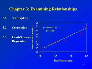
Chapter 3: Examining Relationships. Section 3.3: Least-Squares Regression. Correlation measures the strength and direction of the linear relationship Least-squares regression Method for finding a line that summarizes that relationship between two variables in a specific setting.

E N D
Section 3.3:Least-Squares Regression • Correlation measures the strength and direction of the linear relationship • Least-squares regression • Method for finding a line that summarizes that relationship between two variables in a specific setting. • Regression line • Describes how a response variable y changes as an explanatory variable xchanges • Used to predict the value of y for a given value of x • Unlike correlation, requires an explanatory and response variable.
Least-squares regression line (LSRL) • If you believe the data show a linear trend, it would be appropriate to try to fit an LSRL to the data • We will use the line to predict y from x, so you want the LSRL to be as close as possible to all the points in the vertical direction • That’s because any prediction errors we make are errors in y, or the vertical direction of the scatterplot Error = actual – predicted
Least-squares regression line (LSRL) • The least squares regression line of y on x is the line that makes the sum of the squares of the vertical distances of the data points from the line as small as possible
Least-squares regression line (LSRL) • The equation for the LSRL is • is used because the equation is representing a prediction of y • To calculate the LSRL you need the means and standard deviations of the two variables as well as the correlation • The slope is b and the y-intercept is a • Every least-squares regression line passes through the point
Example 1 – finding the lsrl • Using the data from example 1 (the number of student absences and their overall grade) in section 3.2, write the least squares line. • r = -.946
Finding the LSRL and Overlaying it on your Scatterplot • Press the STAT key • Scroll over to CALC • Use option 8 • After the command is on your home screen: • Put the following L1, L2, Y1 • To get Y1, press VARS, Y-VARS, Function • Press enter • The equation is now stored in Y1 • Press zoom 9 to see the scatterplot with the LSRL
Use the LSRL to Predict • With an equation stored on the calculator it makes it easy to calculate a value of y for any known x. • Using the trace button • 2nd Trace, Value • x = 18 • Using the table • 2nd Graph • Go to 2nd window if you need change the tblstart • Example 2 - • Use the LSRL to predict the overall grade for a student who has had 18 absences. Also, interpret the slope and intercept of the regression line. • A student who has had 18 absences is predicted to have an overall grade of about 14% • The slope is -4.81 which in terms of this scenario means that for each day that a student misses, their overall grade decreases about 4.81 percentage points • The intercept is at 101.04 which means that a student who hasn’t missed any days is predicted to have a grade of about 101%.
The role of r2 in regression. • Coefficient of determination • The proportion of the total sample variability that is explained by the least-squares regression of y on x • It is the square of the correlation coefficient (r), and is therefore referred to as r2 • In the student absence vs. overall grade example, the correlation was r = -.946 • The coefficient of determination would be r2 = .8949 • This means that about 89% of the variation in y is explained by the LSRL • In other words, 89% of the data values are accounted for by the LSRL
Facts about least-squares regression • Distinction between explanatory and response variables is essential • If we reversed the roles of the two variables, we get a different LSRL • There is a close connection between correlation and the slope of the regression line • A change of one standard deviation in x corresponds to rstandard deviations in y • The LSRL always passes through the point • We can describe regression entirely in terms of basic descriptive measures • The coefficient of determination is the fraction of the variation in values of y that is explained by the least-squares regression of y on x
Residuals • Residuals • Deviations from the overall pattern • Measured as vertical distances • Difference between an observed value of the response variable and the value predicted by the regression line Residual = Observed y – predicted y • The mean of the least-squares residuals is always zero • If you round the residuals you will end up with a value very close to zero • Getting a different value due to rounding is known as roundoff error
Residual plot • A residual plot is a scatterplot of the regression residuals against the explanatory variable • Residual plots help us assess the fit of a regression line • Below is a residual plot that shows a linear model is a good fit to the original data • Reason • There is a uniform scatter of points
Residual plot • Below are two residual plots that show a linear model is not a good fit to the original data • Reasons • Curved pattern • Residuals get larger with larger values of x
Influential observations: • Outlier • An observation that lies outside the overall pattern in the y direction of the other observations. • Influential Point • An observation is influential if removing it would markedly change the result of the LSRL • Are outliers in the x direction of a scatterplot • Have small residuals, because they pull the regression line toward themselves. • If you just look at residuals, you will miss influential points. • Can greatly change the interpretation of data.
Location of Influential observations • Child 19 • Outlier • Child 18 • Influential Point
See all of the residuals at once • The calculator calculates the residuals for all points every time it runs a linear regression command • To see this, press 2nd STAT and under NAMES scroll down to RESID • The residuals will be in the order of the data