Download
1 / 29
320 likes | 516 Views
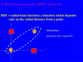
Radial Basis Function Networks. Why network models beyond MLN?. MLN is already universal, but… MLN can have many local minimums. It is often to slow to train MLN. Sometimes, it is extremely difficult to optimize the structure of MLN. There may exist other network architectures….

E N D
Why network models beyond MLN? • MLN is already universal, but… • MLN can have many local minimums. • It is often to slow to train MLN. • Sometimes, it is extremely difficult to optimize the structure of MLN. • There may exist other network architectures…
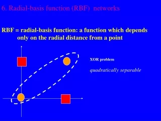
The idea of RBFNN (1) • MLN is one way to get non-linearity. The other is to use • the generalized linear discriminate function, • For Radial Basis Function (RBF), the basis function is radial • symmetry with respect to input, whose value is determined by the • distance from the data point to the RBF center. • For instance, the Gaussian RBF
The idea of RBFNN (2) • For RBFNN, we expect that the function to be learned can be • expressed as a linear superposition of a number of RBFs. The function is described as a linear superposition of three basis functions.
The RBFNN (1) y • RBFNN: a two-layer network w f RBF distance x • Free parameters • --the network weights w in the 2nd layer • --the form of basis functions • --the number of basis functions • --the location of basis functions. • E.g.: for Gaussian RBFNN, they are the number, the centers and the widths • of basis functions
The RBFNN (2) • Universal approximation: for Gaussian RBFNN, it is capable to • approximate any function. • The type of basis functions localized Non-localized
Exact Interpolation • The idea of RBFNN is that we ‘interpolate’ the target function by using the sum of a • number of basis functions. • To illustrate this idea, we consider a special case of exact interpolation, in which the • number of basis functions M is equal to the number of data points N (M=N) and all • basis functions are centered at data points. We want the target values are exactly • interpolated by the summation of basis functions, i.e, • Since M=N, F is a square matrix and is non-singular for general cases, the result is
An example of exact interpolation • For Gaussian RBF (1D input) • 21 data points are generated by y=sin(px) plus noise (strength=0.2) The target data points are indeed exactly interpolated, but the generalization performance is not good.
Beyond exact interpolation • The number of basis functions need not to be equal to the number • data points. Actually, in a typical situation, M should be much • less than N. • The centers of basis functions are no longer constrained to be • at the input data points. Instead, the determination of centers • becomes part of the training process. • Instead of having a common width parameter s, each basis • function can has its own width, which is also to be determined • by learning.
An example of RBFNN RBFNN, 4 basis functions, s=0.4 Exact interpolation, s=0.1
An example of regularization Exact interpolation, s=0.1 With weight decay regularization, n=2.5
The hybrid training procedure • Unsupervised learning in the first layer. This is to fix the basis • functions by only using the knowledge of input data. For Gaussian • RBF, it often includes to decide the number, locations and the • width of RBF. • Supervised learning in the second layer. This is to determine the • network weights in the second layer. If we choose the sum-of-square • error, it becomes a quadratic function optimization, which is easy • to solve. • In summary, the hybrid training avoid to use supervised learning • simultaneously in two layers, and greatly simplify the computational • cost.
Basis function optimization • The form of basis function is predefined, and is often chosen to be • Gaussian. • The number of basis function has often to be determined by trials, • e.g, though monitoring the generalization performance. • The key issue in unsupervised learning is to determine the locations • and the widths of basis functions.
Algorithms for basis function optimization • Subsets of data points. • To randomly select a number of input data points as basis functions centers. • The width can be chosen to be equal and to be given by some multiple of the • average distance between the basis function centers. • Gaussian mixture models. • The choice of basis functions is essentially to model the density distribution of • input data (intuitively we want the centers of basis functions to be at high density • regions). We may assume input data is generated by a mixture of Gaussian • distribution. Optimizing the probability density model returns the basis function • centers and widths. • Clustering algorithms. • In this approach the input data is assumed to consist of a number of clusters. • Each cluster corresponds to one basis function, with the center being the • basis function center. The width can be set to be equal to some multiple of the • average distance between all centers.
K-means clustering algorithm (1) • The algorithm partitions data points into K disjoint subsets (K is predefined). • The clustering criteria are: • -the cluster centers are set in the high density regions of data • -a data point is assigned to the cluster with which it has the minimum distance to • the center • Mathematically, this is equivalent to minimizing the sum-of-square • clustering function,
K-means clustering algorithm (2) • The algorithm Step 1: Initially randomly assign data points to one of K clusters. Each data points will then have a cluster label. Step 2: Calculate the mean of each cluster C. Step 3:Check whether each data pointed has the right cluster label. For each data point, calculate its distances to all K centers. If the minimum distance is not the value for this data point to its cluster center, the cluster identity of this data point will then be updated to the one that gives the minimum distance. Step 4: After each epoch checking (one turn for all data points), if no updating occurs, i.e, J reaches the minimum value, then stop. Otherwise, go back to step 2.
An example of data clustering Before clustering After clustering
The network training • The network output after clustering • The sum-of-square error which can be easily solved.
An example of time series prediction • We will show an example of using RBFNN for time series prediction. • Time series prediction: to predict the system behavior based on its history. • Suppose the time course of a system is denoted as • {S(1),S(2),…S(n)}, where S(n) is the system state at time step n. • the task is to predict the system behavior at n+1 based on the knowledge of • its history. i.e., {S(n),S(n-1),S(n-2),…}. This is possible for many problems • in which system states are correlated over time. • Consider a simple example, the logistic map, in which the system state x • is updated iteratively according to Our task is to predict the value of x at any step based on its values in the previous two steps, i.e., to estimate based on and xn-1 xn-2 xn
Generating training data from the logistic map • The logistic map, though is simple, shows many interesting behaviors. • (more detail can be found at http://mathworld.wolfram.com/LogisticMap.html) • The data collecting process: • --Choose r=4, andthe initial value of x to be 0.3 • --Iterate the logistic map 500 steps, and collect 100 examples from the last • 100 iterations (chopping data into triplets, each triplet gives one • input-output pair). The input data space The time course of the system state
Clustering the input data • We cluster the input data by using the K-means clustering algorithm. • We choose K=4. The clustering result returns the centers of basis functions • and the scale of width. • An typical example
Comparison with multi-layer perceptron (1) • RBF: • Simple structure: one hidden layer, • linear combination at the output layer • Simple training: the hybrid training: • clustering + the quadratic error function • Localized representation: the input space • is covered by a number of localized • basis functions. A given input typically • only activate significantly a limited • number of hidden units (those are within • a close distance) • MLP: • Complicated structure: often many • layers and many hidden units • Complicated training: optimizing • multiple layer together, local minimum • and slow convergence. • Distributed representation: for a given • input, typically many hidden units will • be activated.
Comparison with MLP (2) • Different ways of interpolating data * * * RBF: data are classified according to clusters MLP: data are classified by hyper-planes.
Shortcomings of RBFNN • Unsupervised learning implies that RBFNN may only achieve • sub-optimal solution, since the training of basis functions does not • consider the information of the output distribution. Example: a basis function is chosen based only on the density of input data, which gives p(x). It does not match the real output function h(x).
Shortcomings of RBFNN Example: the output function is only determined by one input component, the other component is irrelevant. Due to unsupervised, RBFNN is unable to detect this irrelevant component, whereas, MLP may do (the network weights connected to irrelevant components will tend to have small values).