Download
1 / 40
420 likes | 568 Views
Radial Basis Function Networks. 20013627 표현아 Computer Science, KAIST. contents. Introduction Architecture Designing Learning strategies MLP vs RBFN. introduction.

E N D
Radial Basis Function Networks 20013627 표현아 Computer Science, KAIST
contents • Introduction • Architecture • Designing • Learning strategies • MLP vs RBFN
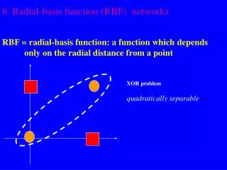
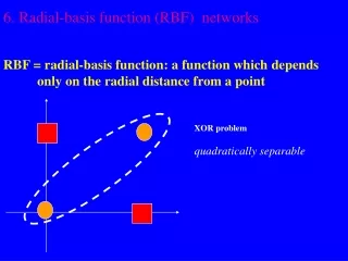
introduction • Completely different approach by viewing the design of a neural network as a curve-fitting (approximation) problem in high-dimensional space ( I.e MLP )
introduction In MLP
introduction In RBFN
introduction Radial Basis Function Network • A kind of supervised neural networks • Design of NN as curve-fitting problem • Learning • find surface in multidimensional space best fit to training data • Generalization • Use of this multidimensional surface to interpolate the test data
introduction Radial Basis Function Network • Approximate function with linear combination of Radial basis functions F(x) = S wi h(x) • h(x) is mostly Gaussian function
architecture h1 x1 W1 h2 x2 W2 h3 x3 W3 f(x) Wm hm xn Input layer Hidden layer Output layer
architecture Three layers • Input layer • Source nodes that connect to the network to its environment • Hidden layer • Hidden units provide a set of basis function • High dimensionality • Output layer • Linear combination of hidden functions
architecture Radial basis function m f(x) = wjhj(x) j=1 hj(x)= exp( -(x-cj)2 / rj2 ) Where cj is center of a region, rj is width of the receptive field
designing • Require • Selection of the radial basis function width parameter • Number of radial basis neurons
designing Selection of the RBF width para. • Not required for an MLP • smaller width • alerting in untrained test data • Larger width • network of smaller size & faster execution
designing Number of radial basis neurons • By designer • Max of neurons = number of input • Min of neurons = ( experimentally determined) • More neurons • More complex, but smaller tolerance
learning strategies • Two levels of Learning • Center and spread learning (or determination) • Output layer Weights Learning • Make # ( parameters) small as possible • Principles of Dimensionality
learning strategies Various learning strategies • how the centers of the radial-basis functions of the network are specified. • Fixed centers selected at random • Self-organized selection of centers • Supervised selection of centers
learning strategies Fixed centers selected at random(1) • Fixed RBFs of the hidden units • The locations of the centers may be chosen randomly from the training data set. • We can use different values of centers and widths for each radial basis function -> experimentation with training data is needed.
learning strategies Fixed centers selected at random(2) • Only output layer weight is need to be learned. • Obtain the value of the output layer weight by pseudo-inverse method • Main problem • Require a large training set for a satisfactory level of performance
learning strategies Self-organized selection of centers(1) • Hybrid learning • self-organized learning to estimate the centers of RBFs in hidden layer • supervised learning to estimate the linear weights of the output layer • Self-organized learning of centers by means of clustering. • Supervised learning of output weights by LMS algorithm.
learning strategies Self-organized selection of centers(2) • k-means clustering • Initialization • Sampling • Similarity matching • Updating • Continuation
learning strategies Supervised selection of centers • All free parameters of the network are changed by supervised learning process. • Error-correction learning using LMS algorithm.
learning strategies Learning formula • Linear weights (output layer) • Positions of centers (hidden layer) • Spreads of centers (hidden layer)
MLP vs RBFN Approximation • MLP : Global network • All inputs cause an output • RBF : Local network • Only inputs near a receptive field produce an activation • Can give “don’t know” output
10.4.7 Gaussian Mixture • Given a finite number of data points xn, n=1,…N, draw from an unknown distribution, the probability function p(x) of this distribution can be modeled by • Parametric methods • Assuming a known density function (e.g., Gaussian) to start with, then • Estimate their parameters by maximum likelihood • For a data set of N vectors c={x1,…, xN}drawn independently from the distribution p(x|q), then the joint probability density of the whole data set c is given by
10.4.7 Gaussian Mixture • L(q) can be viewed as a function of q for fixed c, in other words, it is the likelihood of q for the given c • The technique of maximum likelihood then set the value of q by maximizing L(q). • In practice, it is often to consider the negative logarithm of the likelihood and to find a minimum of E. • For normal distribution, the estimated parameters can be found by analytic differentiation of E:
10.4.7 Gaussian Mixture • Non-parametric methods • Histograms • An illustration of the histogram approach to density estimation. The set of 30 sample data points are drawn from the sum of two normal distribution, with means 0.3 and 0.8, standard deviations 0.1 and amplitudes 0.7 and 0.3 respectively. The original distribution is shown by the dashed curve, and the histogram estimates are shown by the rectangular bins. The number M of histogram bins within the given interval determines the width of the bins, which in turn controls the smoothness of the estimated density.
10.4.7 Gaussian Mixture • Density estimation by basis functions, e.g., Kenel functions, or k-nn (a) kernel function, (b) K-nn Examples of kernel and K-nn approaches to density estimation.
10.4.7 Gaussian Mixture • Discussions • Parametric approach assumes a specific form for the density function, which may be different from the true density, but • the density function can be evaluated rapidly for new input vectors • Non-parametric methods allows very general forms of density functions, thus the number of variables in the model grows directly with the number of training data points. • The model can not be rapidly evaluated for new input vectors • Mixture model is a combine of both: (1) not restricted to specific functional form, and (2) yet the size of the model only grows with the complexity of the problem being solved, not the size of the data set.
10.4.7 Gaussian Mixture • The mixture model is a linear combination of component densities p(x| j ) in the form
10.4.7 Gaussian Mixture • The key difference between the mixture model representation and a true classification problem lies on the nature of the training data, since in this case we are not provided with any “class labels” to say which component was responsible for generating each data point. • This is so called the representation of “incomplete data” • However, the technique of mixture modeling can be applied separately to each class-conditional density p(x|Ck) in a true classification problem. • In this case, each class-conditional density p(x|Ck) is represented by an independent mixture model of the form
10.4.7 Gaussian Mixture • Analog to conditional densities and using Bayes’ theorem, the posterior Probabilities of the component densities can be derived as • The value of P(j|x) represents the probability that a component j was responsible for generating the data point x. • Limited to the Gaussian distribution, each individual component densities are given by : • Determine the parameters of Gaussian Mixture methods: (1) maximum likelihood, (2) EM algorithm.
10.4.7 Gaussian Mixture Representation of the mixture model in terms of a network diagram. For a component densities p(x|j), lines connecting the inputs xi to the component p(x|j) represents the elements mji of the corresponding mean vectors mj of the component j.
Maximum likelihood • The mixture density contains adjustable parameters: P(j), mjand sj where j=1, …,M. • The negative log-likelihood for the data set {xn} is given by: • Maximizing the likelihood is then equivalent to minimizing E • DifferentiationEwith respect to • the centres mj : • the variances sj :
Maximum likelihood • Minimizing of E with respect toto the mixing parametersP(j), must subject to the constraints S P(j)=1, and 0< P(j)<1.Thiscan be alleviated by changing P(j) in terms a set of M auxiliary variables {gj} such that: • The transformation is called the softmax function, and • the minimization of E with respect togj is • using chain rule in the form • then,
Maximum likelihood • Setting we obtain • Setting • Setting • These formulas give some insight of the maximum likelihood solution, they do not provide a direct method for calculating the parameters, i.e., these formulas are in terms of P(j|x). • They do suggest an iterative scheme for finding the minimal of E
Maximum likelihood • we can make some initial guess for the parameters, and use these formula to compute a revised value of the parameters. • Then, using P(j|xn) to estimate new parameters, • Repeats these processes until converges
The EM algorithm • The iteration process consists of (1) expectation and (2) maximization steps, thus it is called EM algorithm. • We can write the change in error of E, in terms of old and new parameters by: • Using we can rewrite this as follows • Using Jensen’s inequality: given a set of numberslj 0, • such that jj=1,
The EM algorithm • Consider Pold(j|x) as lj, then the changes of E gives • Let Q = , then , and is an upper bound of Enew. • As shownin figure, minimizing Q will lead to a decrease of Enew, unless Enew is already at a local minimum. Schematic plot of the error function E as a function of the new value new of one of the parameters of the mixture model. The curve Eold + Q(new) provides an upper bound on the value of E (new) and the EM algorithm involves finding the minimum value of this upper bound.
The EM algorithm • Let’s drop terms in Q that depends on only old parameters, and rewrite Q as • the smallest value for the upper bound is found by minimizing this quantity • for the Gaussian mixture model, the quality can be • we can now minimize this function with respect to ‘new’ parameters, and they are:
The EM algorithm • For the mixing parameters Pnew (j), the constraint SjPnew (j)=1 can be considered by using the Lagrange multiplier l and • minimizing the combined function • Setting the derivative of Z with respect to Pnew (j) to zero, • using SjPnew (j)=1 and SjPold (j|xn)=1, we obtain l = N, thus • Since theSjPold (j|xn) term is on the right side, thus this results are ready for iteration computation • Exercise 2: shown on the nets