Download
1 / 18
330 likes | 887 Views
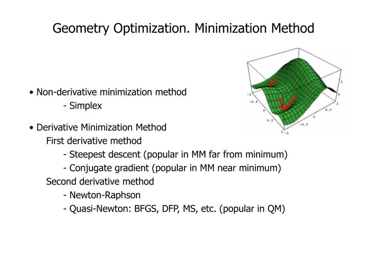
Geometry Optimization. Minimization Method. Non-derivative minimization method - Simplex Derivative Minimization Method First derivative method - Steepest descent (popular in MM far from minimum) - Conjugate gradient (popular in MM near minimum) Second derivative method

E N D
Geometry Optimization. Minimization Method • Non-derivative minimization method • - Simplex • Derivative Minimization Method • First derivative method • - Steepest descent (popular in MM far from minimum) • - Conjugate gradient (popular in MM near minimum) • Second derivative method • - Newton-Raphson • - Quasi-Newton: BFGS, DFP, MS, etc. (popular in QM)
A B R Potential Energy Curve (1-Dimensional) E = E(R) Simplest form: Harmonic Oscillator Simplified
Second derivative method: Newton-Raphson (1D, Diatom) End up with the minimum closest to the input structure (local minimum): No guarantee for the global minimum Constant only when quadratic Optimized in one step, if quadratic, from 1st and 2nd derivatives of energy True only near equilibrium structure Otherwise, optimized in several steps
Second derivative method: Newton-Raphson/Quasi-Newton 1-Dim (diatom; N=2; #(degree of freedom)=3N-5=1) from 1st and 2nd derivatives of energy N-atom; #(degree of freedom)=3N or 3N-6 (non-linear) or 3N-5 (linear) Position (coordinates): 3N-dim. vector 1st derivative (gradient): 3N-dim. vector (easily calculated analytically) 2nd derivative (hessian): 3N3N matrix - inverted (updated at each step analytically or numerically) (time- and memory-consuming for large systems) • Takes only few steps to converge near minimum, but can be unstable far from minimum • Used for small molecules near minimum (after the first steps of steepest descent)
Second derivative method: Newton-Raphson Summary • First derivative gives direction of vector. • Second derivative gives curvature of the direction vector. • This allows for the minimum to be guessed along the line searched. • The minimum of a quadratic function can be reached in one step. • However, energy surface is not quadratic. • Minimum energy cannot be determined with one Newton-Raphson step. • Apply the procedure iteratively. • Pros: • Converges quickly near a minimum (where quadratic) • Requires few energy function calculations • Cons: • Unstable far from a minimum • For large systems the inversion of Hessian becomes intractable. • Large storage requirements
Second derivative method: Quasi-Newton (BFGS) • Does not calculate the inverse Hessian matrix. • Start with guess Hessian and update the Hessian after each step • to form a more accurate Hessian. • Pros: • Avoids calculating the Hessian • Requires few energy calculations • Cons: • Requires storage proportional to N2 • Inefficient in regions where the second derivative changes rapidly
start First derivative method: Steepest descent • Uses 1st derivative to locate the general direction of the minimum. • Uses line searching along a given direction to find structure of lower energy. • The next direction of movement is orthogonal to the previous one. Example
First derivative method: Steepest descent • Pros: • Does not require initial structure to be near the minimum. • Good for minimizing initial structures • – Relieves highest-energy features in a structure. • Cons: • Slow to converge (very slow at low gradient values (near minima)) • Information about previous steps is lost. • Near the minimum the minimization overshoots the minimum point. • Requires large number of energy evaluations.
First derivative method: Conjugate gradient • Increases the efficiency by controlling the choice of new direction • (Fletcher-Reeves model) • Pros: • Quicker to converge for large molecules • Requires less iterations • Cons: • Unstable far from a local minimum. • Requires more function evaluations in a line search (more complete) Example
When to use various minimization methods • Steepest descent: used for initial minimization (10-100 steps) • Conjugate gradient, Newton-Raphson: used to complete the minimization Convergence criteria
for all q Normal mode analysis: Vibration frequencies 1D (diatom) near stationary point >0 for minima <0 for TS frequency (in cm1) real for minima imaginary for TS N-atom (3N-6 dim) minimum: All real frequencies for all q for only one q (reaction coordinate) TS: One imaginary frequencies for other q’s Characterize stationary points from the number of imaginary frequencies
minimum: All real frequencies for all q for only one q (reaction coordinate) TS: One imaginary frequencies for other q’s
Normal mode analysis: Vibration frequencies • Obtain/interpret vibrational spectra (IR, Raman, HREELS, etc) • Obtain zero-point energy • Obtain thermodynamic quantities (enthalpy, entropy, free energy, etc.)