Download
1 / 14
140 likes | 343 Views
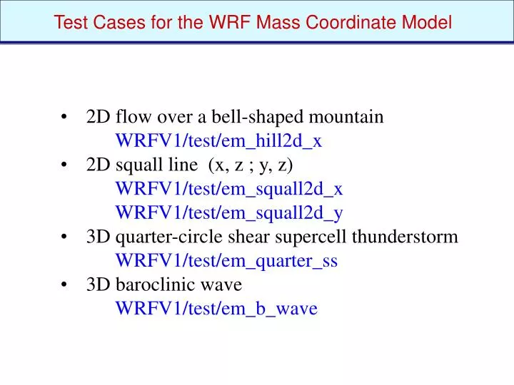
Test Cases for the WRF Mass Coordinate Model. 2D flow over a bell-shaped mountain WRFV1/test/em_hill2d_x 2D squall line (x, z ; y, z) WRFV1/test/em_squall2d_x WRFV1/test/em_squall2d_y 3D quarter-circle shear supercell thunderstorm WRFV1/test/em_quarter_ss 3D baroclinic wave

E N D
Test Cases for the WRF Mass Coordinate Model • 2D flow over a bell-shaped mountain • WRFV1/test/em_hill2d_x • 2D squall line (x, z ; y, z) • WRFV1/test/em_squall2d_x • WRFV1/test/em_squall2d_y • 3D quarter-circle shear supercell thunderstorm • WRFV1/test/em_quarter_ss • 3D baroclinic wave • WRFV1/test/em_b_wave
2D Flow Over a Bell-Shaped Mountain To run: From WRFV1 -compile em_hill2d_x ; From WRFV1/test/em_hill2d_x – run ideal.exe, run wrf.exe Initialization code is in WRFV1/dyn_em/module_initialize_hill2d_x.F The terrain profile is set in the initialization code. The thermodynamic sounding and the initial wind field is read from the ascii file WRFV1/test/em_hill2d_x/input_sounding The 2D solution is computed by integrating the 3D model with 3 points in periodic direction y; without an initial perturbation in y the solution remains y-independent.
Setting the terrain heights In WRFV1/dyn_em/module_initialize_hill2d_x.F SUBROUTINE init_domain_rk ( grid, & ... hm = 100. xa = 5.0 icm = ide/2 ... DO j=jts,jte DO i=its,ite ! flat surface !! ht(i,j) = 0. ht(i,j) = hm/(1.+(float(i-icm)/xa)**2) ! ht(i,j) = hm1*exp(-(( float(i-icm)/xa1)**2)) & ! *( (cos(pii*float(i-icm)/xal1))**2 ) phb(i,1,j) = g*ht(i,j) php(i,1,j) = 0. ph0(i,1,j) = phb(i,1,j) ENDDO ENDDO mountain height and half-width mountain position in domain (central gridpoint in x) Set height field lower boundary condition
Sounding File Format File: WRFV1/test/em_quarter_ss/input_sounding surface Pressure (mb) surface potential Temperature (K) Surface vapor mixing ratio (g/kg) line 1 1000.00 300.00 14.00 250.00 300.45 14.00 -7.88 -3.58 750.00 301.25 14.00 -6.94 -0.89 1250.00 302.47 13.50 -5.17 1.33 1750.00 303.93 11.10 -2.76 2.84 2250.00 305.31 9.06 0.01 3.47 2750.00 306.81 7.36 2.87 3.49 3250.00 308.46 5.95 5.73 3.49 3750.00 310.03 4.78 8.58 3.49 4250.00 311.74 3.82 11.44 3.49 4750.00 313.48 3.01 14.30 3.49 each successive line is a point in the sounding height (m) potential temperature (K) vapor mixing ratio (g/kg) U (west-east) velocity (m/s) V (south-north) velocity (m/s)
2D squall line simulation squall2d_x is (x,z), squall2d_y is (y,z); both produce the same solution. To run: From WRFV1 -compile em_squall2d_x ; From WRFV1/test/em_squall2d_x – run ideal.exe, run wrf.exe Initialization code is in WRFV1/dyn_em/module_initialize_squall2d_x.F This code also introduces the initial perturbation. The thermodynamic sounding and hodograph is in the ascii input file WRFV1/test/em_squall2d_x/input_sounding
3D supercell simulation Height coordinate model (dx = dy = 2 km, dz = 500 m, dt = 12 s, 160 x 160 x 20 km domain ) Surface temperature, surface winds and cloud field at 2 hours
3D supercell simulation To run: From WRFV1 -compile em_quarter_ss ; From WRFV1/test/em_quarter_ss – run ideal.exe, run wrf.exe Initialization code is in WRFV1/dyn_em/module_initialize_quarter_ss.F The thermodynamic sounding and hodograph is read from the ascii input file WRFV1/test/em_quarter_ss/input_sounding The initial perturbation (warm bubble) is hardwired in the initialization code.
Setting the initial perturbation In WRFV1/dyn_em/module_initialize_quarter_ss.F SUBROUTINE init_domain_rk ( grid, & ... ! thermal perturbation to kick off convection write(6,*) ' nxc, nyc for perturbation ',nxc,nyc write(6,*) ' delt for perturbation ',delt DO J = jts, min(jde-1,jte) yrad = dy*float(j-nyc)/10000. ! yrad = 0. DO I = its, min(ide-1,ite) xrad = dx*float(i-nxc)/10000. ! xrad = 0. DO K = 1, kte-1 ! put in preturbation theta (bubble) and recalc density. note, ! the mass in the column is not changing, so when theta changes, ! we recompute density and geopotential zrad = 0.5*(ph_1(i,k,j)+ph_1(i,k+1,j) & +phb(i,k,j)+phb(i,k+1,j))/g zrad = (zrad-1500.)/1500. RAD=SQRT(xrad*xrad+yrad*yrad+zrad*zrad) IF(RAD <= 1.) THEN T_1(i,k,j)=T_1(i,k,j)+delt*COS(.5*PI*RAD)**2 T_2(i,k,j)=T_1(i,k,j) qvf = 1. + 1.61*moist_1(i,k,j,P_QV) alt(i,k,j) = (r_d/p1000mb)*(t_1(i,k,j)+t0)*qvf* & (((p(i,k,j)+pb(i,k,j))/p1000mb)**cvpm) al(i,k,j) = alt(i,k,j) - alb(i,k,j) ENDIF ENDDO horizontal radius of the perturbation is 10 km, centered at (x,y) gridpoints (nxc, nyc) vertical radius of the perturbation is 1500 m perturbation added to initial theta field maximum amplitude of the perturbation
Moist Baroclinic Wave Simulation Height coordinate model (dx = 100 km, dz = 250 m, dt = 600 s) Surface temperature, surface winds, cloud and rain water
Open Channel Baroclinic Wave Simulation Day 5 dt = 600 s dx = dy = 100 km 14000 x 8000 km Free Slip Warm Rain MRF PBL - land KF Conv. Param. Ice MIcrophysics
Moist Baroclinic Wave Simulation To run: From WRFV1 -compile em_b_wave ; From WRFV1/test/em_b_wave – run ideal.exe, run wrf.exe Initialization code is in WRFV1/dyn_em/module_initialize_b_wave.F The initial jet (y,z) is read from the binary input file WRFV1/test/em_b_wave/input_jet The initial perturbation is hardwired in the initialization code.
Moist Baroclinic Wave Simulation Default configuration in WRFV1/test/em_b_wave/namelist.input runs the dry jet in a periodic channel with dimension (4000 x 8000 x 16 km) (x,y,z). Turning on any microphysics (mp_physics > 0 in namelist.input) puts moisture into the basic state. Switching from periodic to open boundary conditions along with lengthening the channel produces a baroclinic wave train. The initial jet only works for dy = 100 km and 81 grid points in the y (south-north) direction.