Inverse Laplace Transform

1. Inverse Laplace Transform

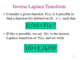
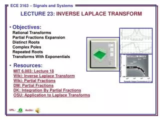
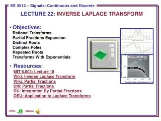
2. Inverse Laplace Transform • Definition has integration in complex plane We will use lookup tables instead Roberts, Appendix F • Many Laplace transform expressions are ratios of two polynomials, a.k.a. rational functions • Convert complicated rational functions into simpler forms Apply partial fractions decomposition Use lookup tables

3. Partial Fractions Example #1

4. Partial Fractions Example #2

5. Partial Fractions Example #3

6. Mathematica • Function Apart performs partial fractions but returns conjugate poles in quadratic form Apart[(2 s^2 + 5)/(s^2 + 3 s + 2), s] • Laplace transform is an add-on package Needs[ “Calculus`Master`” ] • Forward Laplace Transform LaplaceTransform[Exp[-a*t], t, s] Note that u(t), which is UnitStep[t], is implied. • Inverse Laplace Transform InverseLaplaceTransform[1/(s+a),s,t] double quote backquote

7. Laplace Transform Properties • Linearity • Time shifting • Frequency shifting • Differentiationin time

8. Differentiation in Time Property

9. Laplace Transform Properties • Differentiation in frequency • Integration in time Example: f(t) = d(t) • Integration in frequency

10. f(2 t) f(t) t t -1 1 -2 2 Laplace Transform Properties • Scaling in time/frequency • Under integration, • Convolution in time • Convolution in frequency Area reduced by factor 2

11. Example • Compute y(t) = e a t u(t) * e b t u(t) , where a b • If a = b, then we would have resonance • What form would the resonant solution take?

12. Linear Differential Equations • Using differentiation in time propertywe can solve differential equations (including initial conditions) using Laplace transforms • Example: y”(t) +5 y’(t) + 6 y(t) = f ’(t) + f(t) With y(0-) = 2, y’(0-) =1, and f(t) = e- 4 t u(t) So f ’(t) = -4 e-4 t u(t) + e-4 t d(t), f ’(0-) = 0 and f ’(0+) = 1 See handout G

13. Mathematica Solution • Define DSolve Needs[ "Calculus`Master`" ]; • Define f(t) and solve for y(t) f[t_] := Exp[-4 t]; DSolve[ { y''[t] + 5 y'[t] + 6 y[t] == D[ f[t], t ] + f[t],y[0] == 2, y'[0] == 1 },y[t], t ] • Does not distinguish between 0- and 0+

14. Initial and Final Values • Values of f(t) as t 0 and t   may be computed from its Laplace transform F(s) • Initial value theorem If f(t) and its derivative df/dt have Laplace transforms, then provided that the limit on the right-hand side of the equation exists. • Final value theorem If both f(t) and df/dt have Laplace transforms, then provided that s F(s) has no poles in right-hand plane or on imaginary axis.

15. Final and Initial Values Example • Transfer function Poles at s = 0, s = -1  j2 Zero at s = -3/2 Initial Value Final Value