Download
1 / 18
180 likes | 316 Views
Mixed layer depth variability and phytoplankton phenology in the Mediterranean Sea. H. Lavigne 1 , F. D’Ortenzio 1 , M. Ribera d’Alcalà 2 , H. Claustre 1 Laboratoire d’Océanographie de Villefranche , France 2. Stazione Zoologica A. Dohrn , Naples, Italy.

E N D
Mixed layer depth variability and phytoplankton phenology in the Mediterranean Sea H. Lavigne1, F. D’Ortenzio1, M. Ribera d’Alcalà2, H. Claustre1 Laboratoire d’Océanographie de Villefranche, France 2. StazioneZoologica A. Dohrn, Naples, Italy 45thLiège Colloquium – May 17th 2013
CONCLUSION INTRODUCTION DISCUSSION RESULTS DATA & METHODS • It is now well recognized that the phytoplankton phenology is impacted by mixed layer depth (MLD) variability (blooms events are good examples). • However, it is still challenging to observe and characterize the impact of MLD on phytoplankton (MLD and phytoplankton biomass change rapidly, low availability of the phytoplankton biomass data). • Merging in situ MLD data and ocean color chlorophyll-a concentration ([Chl]SAT) data represents a way to explore interactions between MLD annual cycle and phytoplankton phenology.
CONCLUSION INTRODUCTION DISCUSSION RESULTS DATA & METHODS Present analysis was performed on the Mediterranean Sea because • Data availability (weak cloud coverage for [Chl]SAT, and important CTD sampling). • contrasting biogeochemical regimes co-exist over the basin. Present analysis was based on : • The generation of concomitant MLD and [Chl]SAT annual cycles. • Spatial averages computed in established bioregions. • Description of MLD and [Chl]SAT cycles based on a new set of metrics.
Data CONCLUSION DATA & METHODS DISCUSSION RESULTS INTRODUCTION Mixed Layer Depth (MLD) calculated from in situ CTD measurements. • Historical database (D’Ortenzio et al. 2005 updated with Coriolis). • 72186 profiles of temperature and salinity • Computation of MLD (criteria in density difference 0.03 kg m-3) Satellite surface chlorophyll-a concentration ([Chl]SAT) The data density is not sufficient to work with a regular mesh grid. A bioregionalization was used instead. • SeaWiFS (1998 – July 2007) et MODIS-Aqua (July 2007 - 2010) • Level 3, 8-day , 9km • Standard NASA algorithm (O’Reilly et al., 2007)
CONCLUSION DATA & METHODS DISCUSSION RESULTS INTRODUCTION The geographicalframework - Starting point the bioregionalization of the MediterraneaSeaproposed by D’Ortenzio and Ribera d’Alcalà (2009). Result from a k-means cluster analysis based on the seasonal cycle of SeaWiFS chlorophyll- a concentration Source: D’Ortenzio et Ribera D’alcalà (2009) 3 mains kinds of dynamics appeared bloom intermittent no bloom
CONCLUSION DATA & METHODS DISCUSSION RESULTS INTRODUCTION Med NW - Bloom bioregion MLD and [Chl]SAT observations Data processing spatial temporal Ionian - No bloom bioregion Generation of concomitant MLD and [Chl]SAT annual cycles at 8-day resolution • Climatological scale • Interannualscale • All MLD and [Chl]SAT observations are mixed to produce a climatological cycle. • Data are averaged for each year separately.
CONCLUSION DATA & METHODS DISCUSSION RESULTS INTRODUCTION Metrics to describe annual MLD and [Chl]SAT cycles CHL-MAX MLD-MAX [Chl]SAT MLD CHL-MAX: annual maximum of [Chl]SAT MLD-MAX: annual maximum of MLD ΔINIT: Time lag between the initiation of mixing and the initiation of [Chl]SAT increase (determination of the initiation date: annual median + 5%; Siegel et al., 2002). ΔMAX: Time lag between the date of MLD maxima and the date of [Chl]SAT maxima. June year n+1 July year n ΔINIT ΔMAX
CONCLUSION DISCUSSION RESULTS DATA & METHODS Med NW - Bloom The climatological scale INTRODUCTION Ionian - No Bloom
CONCLUSION DISCUSSION RESULTS DATA & METHODS Med NW - Bloom The interannual scale : the analysis of annual cycles INTRODUCTION • The shape of MLD and [Chl]SAT cycles vary from year to year. • For 4 cycles out of 5, the succession MLD deepening followed by [Chl]SAT increase and decay is repeated. • Cycle 2006/2007 is anomalous. Ionian – No Bloom • The shape of MLD and [Chl]SAT cycles are fairly similar to the climatology. • The absolute values, especially for MLD and [Chl]SAT peaks, are variable.
The interannual scale: the analysis of metrics CONCLUSION DISCUSSION RESULTS DATA & METHODS INTRODUCTION • The metric MLD-MAX is highly variable, by comparison to CHL-MAX. • MLD-MAX and CHL-MAX are both higher in the “Bloom” bioregion than in the “No Bloom” bioregion. • ΔINIT is relatively stable and similar for the “Bloom” and “No Bloom” bioregions. • ΔMAX is more variable, especially for the “No Bloom” bioregion. • ΔMAX is higher for the “Bloom” than for the “No Bloom” bioregion.
Summary CONCLUSION DISCUSSION RESULTS DATA & METHODS • Metrics are a powerful tool to identify patterns in the MLD and [Chl]SAT cycles. • These patterns are relatively consistent between interannual and climatological analyses. • Metrics analysis confirmed that in the Mediterranean Sea stronger biomass accumulation matches with areas where winter MLDs are the deepest. • Metrics analysis revealed temporal differences between main MLD and [Chl]SAT events (measured with ΔINIT and ΔMAX). How we can explain the ΔMAX difference and the ΔINIT of 30 days? INTRODUCTION
Do light and nutrient availability can explain the ΔINIT and ΔMAX values in the « Bloom » and « No Bloom » bioregions? CONCLUSION DISCUSSION DATA & METHODS PrNUT PrLIGHT • Probability that the MLD is deeper than the nitracline depth. • Empirical estimation (MLD and nitracline datasets are confronted) • Nitracline data set: • Nitracline = isoline 1µM • Calculated from a dataset of 5318 nitrates profiles (MEDAR, SESAME projects). • Probability that the MLD is above the critical depth (Dcr, Sverdrup 1953). • Empirical estimation (MLD dataset is compared to a climatological estimation of the critical depth, calculation method Siegel et al. 2002) INTRODUCTION RESULTS 1.3 mol photon m-2 d-1 SeaWiFSclimatology
Do light and nutrient availability can explain the ΔINIT and ΔMAX values in the « Bloom » and « No Bloom » bioregions? CONCLUSION DISCUSSION DATA & METHODS Med NW - Bloom Ionian – No Bloom PrNUT INTRODUCTION RESULTS Med NW - Bloom Ionian – No Bloom PrLIGHT
CONCLUSION DATA & METHODS ΔMAX ♦ BLOOM: ~ 30 days ♦NO BLOOM : ~ 0 days Hypothesis: Episodically, a deficit of light could limit the growth during winter. INTRODUCTION Hypothesis: [Chl]SAT increase only when the MLD is below the nitracline (November) RESULTS Hypothesis: Light is always available and irregular nutrients supplies by mixing sustain phytoplankton growth during winter. DISCUSSION ΔINIT ♦ BLOOM : ~ 30 days ♦NO BLOOM : ~ 30 days
Conclusions and Perspectives CONCLUSION DATA & METHODS • Metrics are a powerful tool to identify phenological patterns and characterize the influence of the mixed layer. • The relevance of metrics ΔINIT and ΔMAX wasemphasized. • In the Mediterranean Sea, we proposed some hypotheses to explain their behaviors. (Lavigne et al. JGR, in revision) • The proposed phenological metrics could be particularly adapted for profiling floats observations. INTRODUCTION RESULTS DISCUSSION
Thanks to FabrizioD’Ortenzio (my supervisor), LoïcHoupert (CEFREM, Perpignan FRANCE) and Rosario Lavezza (SZN, Napoli, Italy) for their help on CTD and nitrate data. Thank you to for your attention Contact: lavigne@obs-vlfr.fr