Download

1 / 30
300 likes | 386 Views
Chapter 11.1 Inference for the Mean of a Population.

E N D
Chapter 11.1 Inference for the Mean of a Population.
Example 1:One concern employers have about the use of technology is the amount of time that employees spend each day making personal use of company technology, such as phone, e-mail, internet, and games. The Associated Press reports that, on average, workers spend 72 minutes a day on such personal technology uses. A CEO of a large company wants to know if the employees of her company are comparable to this survey. In a random sample of 10 employees, with the guarantee of anonymity, each reported their daily personal computer use. The times are recorded at right. When the standard deviation of a statistic is estimated from the data, the result is called the standard errorof the statistic, and is given by s/√n. When we use this estimator, the statistic that results does not have a normal distribution, instead it has a new distribution, called the t-distribution. Does the data provide evidence that the mean for this company is greater than 72 minutes? What is different about this problem?
One-Sample z-statistic s known: m z =
One-sample t-statistic: s unknown: m t =
The variability of the t-statistic is controlled by the Sample Size. The number of degrees of freeomis equal to n-1 .
ASSUMING NORMALITY? • SRS is extremely important. • Check for skewness. • Check for outliers. • If necessary, make a cautionary statement. • In Real-Life, statisticians and researchers try very hard to avoid small samples. Use a Box and Whisker to check.
Example 2: The Degree of Reading Power (DRP) is a test of the reading ability of children. Here are DRP scores for a random sample of 44 third-grade students in a suburban district: 40 26 39 14 42 18 25 43 46 27 19 47 19 26 35 34 15 44 40 38 31 46 52 25 35 35 33 29 34 41 49 28 52 47 35 48 22 33 41 51 27 14 54 45 At the a = .1, is there sufficient evidence to suggest that this district’s third graders reading ability is different than the national mean of 34?
H0: m = 34 where m is the true mean reading Ha: m = 34 ability of the district’s third-graders SRS? • I have an SRS of third-graders Normal? How do you know? • Since the sample size is large, the sampling distribution is approximately normally distributed • OR • Since the histogram is unimodal with no outliers, the sampling distribution is approximately normally distributed Name the Test!! One Sample t-test for mean Do you know s? What are your hypothesis statements? Is there a key word? • sis unknown Plug values into formula. p-value = tcdf(.6467,1E99,43)=.2606(2)=.5212 Use tcdf to calculate p-value. a = .1
Compare your p-value to a & make decision Conclusion: Since p-value > a, I fail to reject the null hypothesis. There is not sufficient evidence to suggest that the true mean reading ability of the district’s third-graders is different than the national mean of 34. Write conclusion in context in terms of Ha.
Back to Example 1. The times are recorded below. Employee 1 2 3 4 5 6 7 8 9 10 Time 66 70 75 88 69 71 71 63 89 86 Does this data provide evidence that the mean for this company is greater than 72 minutes?
SRS? • I have an SRS of employees • Since the histogram has no outliers and is roughly symmetric, the sampling distribution is approximately normally distributed Normal? How do you know? Do you know s? What are your hypothesis statements? Is there a key word? • sis unknown, therefore we are using a 1 sample t-test H0: m = 72 where m is the true # of min spent on PT Ha: m = 72 time spent by this company’s employees Use tcdf to calculate p-value. Plug values into formula. p-value = tcdf(.937,1E99,9)=.1866(2)=.3732
Compare your p-value to a & make decision Conclusion: Since p-value > 15%, I fail to reject the null hypothesis that this company’s employees spend 72 minutes on average on Personal Technology uses. There is not sufficient evidence to suggest that the true amount of time spent on personal technology use by employees of this company is more than the national mean of 72 min. Write conclusion in context in terms of Ha.
Example 3: The Wall Street Journal (January 27, 1994) reported that based on sales in a chain of Midwestern grocery stores, President’s Choice Chocolate Chip Cookies were selling at a mean rate of $1323 per week. Suppose a random sample of 30 weeks in 1995 in the same stores showed that the cookies were selling at the average rate of $1208 with standard deviation of $275. Does this indicate that the sales of the cookies is different from the earlier figure?
Assume: • Have an SRS of weeks • Distribution of sales is approximately normal due to large sample size • s unknown • H0: m = 1323 where m is the true mean cookie sales • Ha: m≠ 1323 per week • Since p-value < a of 0.05, I reject the null hypothesis. There is sufficient to suggest that the sales of cookies are different from the earlier figure. Name the Test!! One Sample t-test for mean
Example 3: President’s Choice Chocolate Chip Cookies were selling at a mean rate of $1323 per week. Suppose a random sample of 30 weeks in 1995 in the same stores showed that the cookies were selling at the average rate of $1208 with standard deviation of $275. Compute a 95% confidence interval for the mean weekly sales rate. CI = ($1105.30, $1310.70) Based on this interval, is the mean weekly sales rate statistically different from the reported $1323?
In a one-sided test, all of a (2%) goes into that tail (lower tail). What do you notice about the decision from the confidence interval & the hypothesis test? Remember your, p-value = .01475 At a = .02, we would reject H0. What decision would you make on Example 3 if a = .01? What confidence level would be correct to use? Does that confidence interval provide the same decision? If Ha: m < 1323, what decision would the hypothesis test give at a = .02? Now, what confidence level is appropriate for this alternative hypothesis? A 96% CI = ($1100, $1316). Since $1323 is not in the interval, we would reject H0. You would fail to reject H0 since the p-value > a. You should use a 99% confidence level for a two-sided hypothesis test at a = .01. The 98% CI = ($1084.40, $1331.60) - Since $1323 is in the interval, we would fail to reject H0. Why are we getting different answers? Tail probabilities between the significant level (a) and the confidence level MUST match!) In a CI, the tails have equal area – so there should also be 2% in the upper tail CI = ($1068.6 , $1346.40) - Since $1323 is in this interval we would fail to reject H0. a = .02 .96 .02 That leaves 96% in the middle & that should be your confidence level
Ex4: The times of first sprinkler activation (seconds) for a series of fire-prevention sprinklers were as follows: 27 41 22 27 23 35 30 33 24 27 28 22 24 Construct a 95% confidence interval for the mean activation time for the sprinklers.
Matched Pairs Test A special type of t-inference
Pair individuals by certain characteristics Randomly select treatment for individual A Individual B is assigned to other treatment Assignment of B is dependent on assignment of A Individual persons or items receive both treatments Order of treatments are randomly assigned or before & after measurements are taken The two measures are dependent on the individual Matched Pairs – two forms
1)A college wants to see if there’s a difference in time it took last year’s class to find a job after graduation and the time it took the class from five years ago to find work after graduation. Researchers take a random sample from both classes and measure the number of days between graduation and first day of employment Is this an example of matched pairs? No, there is no pairing of individuals, you have two independent samples
2) In a taste test, a researcher asks people in a random sample to taste a certain brand of spring water and rate it. Another random sample of people is asked to taste a different brand of water and rate it. The researcher wants to compare these samples Is this an example of matched pairs? No, there is no pairing of individuals, you have two independent samples – If you would have the same people taste both brands in random order, then it would be an example of matched pairs.
3) A pharmaceutical company wants to test its new weight-loss drug. Before giving the drug to a random sample, company researchers take a weight measurement on each person. After a month of using the drug, each person’s weight is measured again. Is this an example of matched pairs? Yes, you have two measurements that are dependent on each individual.
A whale-watching company noticed that many customers wanted to know whether it was better to book an excursion in the morning or the afternoon. To test this question, the company collected the following data on 15 randomly selected days over the past month. (Note: days were not consecutive.) You may subtract either way – just be careful when writing Ha Since you have two values for each day, they are dependenton the day – making this data matched pairs First, you must find the differences for each day.
I subtracted: Morning – afternoon You could subtract the other way! • Assumptions: • Have an SRS of days for whale-watching • s unknown • Since the boxplot doesn’t show any outliers, we can assume the distribution is approximately normal. You need to state assumptions using the differences! Notice the skewness of the boxplot, however, with no outliers, we can still assume normality!
Is there sufficient evidence that more whales are sighted in the afternoon? Be careful writing your Ha! Think about how you subtracted: M-A If afternoon is more should the differences be + or -? Don’t look at numbers!!!! If you subtract afternoon – morning; then Ha: mD>0 H0: mD = 0 Ha: mD < 0 Where mD is the true mean difference in whale sightings from morning minus afternoon Notice we used mD for differences & it equals 0 since the null should be that there is NO difference.
finishing the hypothesis test: Since p-value > a, I fail to reject H0. There is insufficient evidence to suggest that more whales are sighted in the afternoon than in the morning. In your calculator, perform a t-test using the differences (L3) Notice that if you subtracted A-M, then your test statistic t = + .945, but p-value would be the same
Ex: The effect of exercise on the amount of lactic acid in the blood was examined in journal Research Quarterly for Exercise and Sport. Eight males were selected at random from those attending a week-long training camp. Blood lactate levels were measured before and after playing 3 games of racquetball, as shown in the table. What is the parameter of interest in this problem? Construct a 95% confidence interval for the mean change in blood lactate level.
Based on the data, would you conclude that there is a significant difference, at the 5% level, that the mean difference in blood lactate level was over 10 points?