Download
1 / 39
390 likes | 740 Views
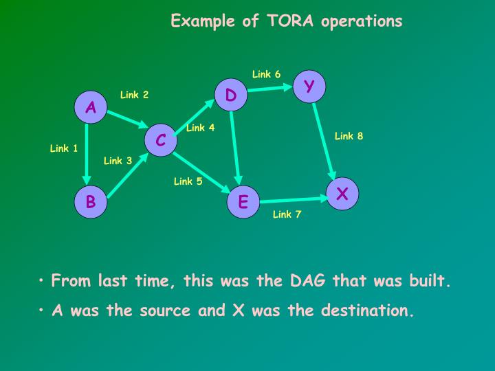
Example of TORA operations. Link 6. Y. D. Link 2. A. Link 4. C. Link 8. Link 1. Link 3. Link 5. X. B. E. Link 7. From last time, this was the DAG that was built. A was the source and X was the destination. Reacting to failures: Route Maintenance. Let Link 4 fail.

E N D
Example of TORA operations Link 6 Y D Link 2 A Link 4 C Link 8 Link 1 Link 3 Link 5 X B E Link 7 • From last time, this was the DAG that was built. • A was the source and X was the destination.
Reacting to failures: Route Maintenance • Let Link 4 fail. • At this time notice that other than the destination all nodes still have an outbound link. • Thus, none of the nodes generate an UPD message. • The DAG is still OK ! • This is especially attractive when the network is dense – most nodes have many outbound links. Link 6 Y D Link 2 A Link 4 C Link 8 Link 1 Link 3 Link 5 X B E Link 7
Let Link 7 fail. • Now, Node E does not have any outbound links ! • Thus, we resort to full link reversal at E. • E generates a new reference level which is 1, sets the oid to E and transmits an UPD message. • It also reverses the direction of all its inbound links. Link 6 Y D Link 2 A C Link 8 Link 1 Link 3 Link 5 X B E Link 7 (1,E,0,0,E)
At this, Node C no longer has outbound links. • It resorts to partial link reversal – reverses the direction of its links to A and B and transmits an UPD. • It also sets its own offset to –1 to ensure that it is at a lower level compared to E. Link 6 Y D Link 2 A (1,E,0,-1,C) C Link 8 Link 1 Link 3 Link 5 X B E
Link 6 Y D Link 2 A • Now the situation repeats at B. • After B reverses its links and transmits an UPDATE. C Link 8 Link 1 Link 3 Link 5 X B E (1,E,0,-2,B)
The situation repeats at A. • This is now a full reversal. A got updates from B and C. • Thus, A stays at the same level as C, but indicates the full reversal by flipping ri. • This causes a partial reversal at B. (1,E,1,-2,A) Link 6 Y D Link 2 A C Link 8 Link 1 Link 3 Link 5 X B E Link 6 Y D Link 2 A C Link 8 Link 1 Link 3 Link 5 X B E (1,E,1,-3,B)
Link 6 Y D Link 2 A (1,E,1,-4,C) C Link 8 Link 1 Link 3 Link 5 X B E • Finally an update is generated at C. • DAG is restored !
Link 6 Y • Now let Link 5 fail. This causes a network partition. • E,D,Y and X are ok. • C has no outbound links. • It creates a new reference level which is 2, and sets the oid to C and sends a UPD. • This causes B to have no outbound links. D Link 2 A C Link 8 Link 1 Link 3 Link 5 X B E Link 6 Y D Link 2 A (2,C,0,0,C) C Link 8 Link 1 Link 3 X B E
B resorts to partial reversal. • It reverses its link to A and broadcasts an update. • Now A does not have outbound links. • It resorts to a full reversal. At full reversal ri is flipped. • This causes a partial reversal at B. (2,C,1,-1,A) Link 2 A Link 2 A C C Link 1 Link 3 Link 1 Link 3 B B (2,C,0,-1,B)
B’s UPD message after the partial reversal creates the same situation at C. • This would cause C to realize that there is no path to X. It sets its height to NULL and sends an UPD to A and B. • Now the nodes realize that there is no path to X. Link 2 A C Link 1 Link 3 B (2,C,1,-2,B) • Important Point : Height is reduced with respect to node that created the reference level.
Advantages: • That of an on-demand routing protocol – create a DAG only when necessary. • Multiple paths created. • Good in dense networks. • Disadvantages • Same as on-demand routing protocols. • Not much used since DSR and AODV outperform TORA. • Not scalable by any means.
References • Chapter 8 of book. • V.D.Park and Scott.M.Corson, “A Highly Adaptive Distributed Routing Algorithm for Mobile Wireless Networks”, Proceedings of INFOCOM 1997.
Associativity Based Routing (ABR) • Proposed by C-K.Toh currently at Georgia Tech. • Introduces a new metric for routing which is called “Degree of Association Stability”. • ABR is free from loops. • What is association stability ? • How stable are nodes with respect to each other ? • Based on an estimate of this, a route is selected.
Each node would periodically generate and transmit a beacon to signify its existence. • Neighboring nodes receive this beacon. • They, maintain what is known as an associativity table. • For each beacon received, the associativity of the receiving node with respect to the beaconing node is incremented. • Thus, to reiterate there is an indication of how stable nodes are with respect to each other. • Association Stability is defined by the connection stability in “time” and “space” of one node with respect to another.
Associativity entries (or ticks as they are called) are reset when the neighbors of a node, or the node itself moves out of proximity. • Goal :? • Longevity – longer lived routes for stability. • Lower Overhead (?) • Three phases of ABR: • Route Discovery • Route Re-construction • Route Deletion • NOW HERE IS A NEW CONCEPT !!!!!!
ROUTE DISCOVERY • Each node broadcasts a query message (BQ message just to sound different ! ) in order to find a destination. • In addition to the address, the associativity ticks with respect to their neighbors is appended. • The receiving node, chooses the best one, i.e., retains only the entry corresponding to itself and its upstream node. • Thus, at the destination, multiple routes are available. • It chooses the one that is best in terms of associativity ticks. • If there is a tie, choose shortest path.
Destination generates a REPLY message towards the source. • Intermediate nodes that forward this message mark the corresponding routes as valid. • Thus, only one route at a given time.
ROUTE MAINTENANCE • Partial route recovery is allowed. • Intermediate nodes will try and rediscover route from point of failure. • When routes are no longer valid, they would be erased. • This is similar to DSR – except for associativity. • In addition partial route discovery.
Advantages: • Tries to find stable routes – lower overhead in some scenarios. • Partial recovery may be faster in some cases. • Disadvantages • Unclear if the overhead incurred in maintaining stability info. is higher than the actual gains. Depends on scenario. • Partial recovery may lead to longer and less stable routes.
References • Chapter 9 on book. • Read about effects of beaconing on battery life. • C-K. Toh, “A Novel Distributed Routing Protocol to support Ad Hoc Mobile Computing”, Proceedings of IEEE 15th Annual International Phoenix Conference on Computers and Communication”, March 1996. • E.Royer and C-K.Toh, “A Review of Current Routing Protocols for Ad-Hoc Mobile Networks”, IEEE Personal Comm. Mag. April 1999.
Signal Stability based Adaptive Routing (SSA) • Prof. Tripathi’s work. • Reference: R.Dube, C.D.Rais, K.Y.Wang and S.K.Tripathi, “Signal Stability based Adaptive Routing for Ad Hoc Mobile Networks”, IEEE Personal Communications Magazine, February 1997.
Principle of SSA • Select routes based on the signal strength between nodes and on a node’s location stability. • Choose routes that have stronger connectivity. • SSA has two component co-operative protocols: • The Dynamic Routing Protocol • The Static Routing Protocol.
The Dynamic Routing Protocol (DRP) • The DRP is responsible for maintaining what is called the Signal Stability Table and also the Routing Table. • SST – record of signal strengths of neighboring nodes which is obtained by means of periodic beaconing. • Quantized levels possible weak channel vs. strong channel. • When a packet is received, DRP processes the packet, updates the tables and passes the received packet to the SRP.
The Static Routing Protocol (DRP) • Forwards the packet up to the transport layer if it is the receiver. • If not, it looks up the routing table and forwards the packet to the appropriate next-hop. • If no entry is found, it initiates a route search.
The Route Search • Route requests are propagated throughout the network – however ... • Forwarded onto the next hop, only if they are received over “strong” channels” and have not yet been previously processed. /* Notice that the second condition prevents looping */. • The destination chooses the first arriving query message because it is most probable that the packet arrived on the “strongest”, shortest and/or least congested path. • DRP reverses the route and sends a route-reply back to the sender.
The PREF field • Notice so far that a route-search packet is forwarded only if it arrived on a strong link. • However, it is possible that no route is found with strong links all the way. • At this time, the source initiates another route-search and uses what is called the “PREF” field to indicate that weak links are acceptable.
Route Maintenance • Use a route error message to the source to indicate which channel has failed. • Source then initiates a new route-search to find a new path to the destination.
Advantages: • More stable routes since signal strength indicates stability. • No overhead incurred in dissemination of tables. • Disadvantages • Of on-demand routing protocols. • The time over which the signal strength is averaged out might be an issue.
Location Aided Routing (LAR) • By Nitin Vaidya and Young-bae Ko. • Reference: “Location Aided Routing (LAR) in Mobile Ad Hoc Networks”, Y.Ko and N.Vaidya, Proceedings of Mobicom 1998. • Idea: Use Location Information for doing Routing – does the name give a hint or what ? • The location info is obtained using GPS (Global Positioning System). • Forward the packet towards the destination instead of forwarding it indiscreetly.
Global Positioning System (GPS) • It is a system that allows a mobile user to know its physical location. • There is however some error in the estimated position. • Different systems have different errors – few meters to about 100 meters.
The notion of expected zone • If a source (S) knows that a destination (D) was at position L at time t0, it has some notion of where the destination might be at a later time t1. • If the average speed of D is v, then S might expect that D is within a circular radius of v (t1-t0) which is centered at L. • However, note that this is only an estimate. If the actual speed was higher, the node might be outside this circle. • This circular region is called the “expected zone”.
Why is the expected zone important ? • If we have an on-demand routing protocol, now we can disseminate a query within the expected zone ! • Note that if there is no information whatsoever with respect to the destination, query search would degenerate to pure flooding. • On the other hand, if we further knew that D was moving north, then the expected zone may be further refined.
The Request Zone • Source node defines what is known as a request zone. • A node would forward the request only if it belongs to the request zone. • Typically, the request zone would include the expected zone. • Additionally nodes in other regions around the expected zone are to be included in the request zone. Why ?
The Request Zone (Continued) • Source node might not belong to the expected zone. Thus, other nodes which are not in the expected zone would need to forward request towards the expected zone. • If with an initial request zone, the destination is not found (because no route exists entirely within the request zone), an expanded request zone may be defined. • In an extreme case, the expanded request zone might be just doing flooding. • There is a tradeoff between latency and message overhead.
Defining the Request Zone Expected Zone • In the first scheme, the suggestion is that the request zone be the rectangle that includes the source and the expected zone of the destination. • Source determines the co-ordinates of the rectangle and includes in query. • A node upon receiving this, will forward the query only if it is within the rectangle. D v(t1-t0) S Request Zone Entire Network
Expected Zone S D v(t1-t0) Request Zone Entire Network • The destination node, Node D would respond with its current location, and current time in its reply message. • It could also include its current speed, or average speed over a recent time interval.
Size of the request zone • Initially destination’s location, D is unknown. • The size of the request zone depends upon the average speed of movement of the destination “v”, and the time elapsed since the last known location of D was recorded. • If v is large, larger expected zone, larger request zone. • If communication with D is infrequent, it may result in a larger request zone. • It may be possible to piggyback location info. on packets other than the query.
A Second Possible Scheme for determining the Request Zone. • Source node knows location (X,Y) of dest at some time t0. It calculates its distance from (X,Y) = Ds. • It includes both, (X,Y) and Ds in the query message. • A node I, forwards it if for some parameter d, if its own distance from the destination DI <= Ds + d. • If this message is further received by node J, node J would forward it only if its distance from the destination DJ <= DI + d. • Obviously the idea is that you try and get closer and closer to the destination. • More details in the paper.
Finally, remember we said GPS could have some error. • Thus, some leeway has to be provided to take this error into account while determining the expected zone and the request zone. • That is my brief intro to ABR, SSA and LAR.