Download
1 / 40
530 likes | 1.04k Views
Spatial statistics. Lecture 3. What are spatial statistics. Not like traditional, a-spatial or non-spatial statistics But specific methods that use distance, space, and spatial relationships as part of the math for their computations It is a spatial distribution and pattern analysis tool

E N D
Spatial statistics Lecture 3
What are spatial statistics • Not like traditional, a-spatial or non-spatial statistics • But specific methods that use distance, space, and spatial relationships as part of the math for their computations • It is a spatial distribution and pattern analysis tool • Identifying characteristics of a distribution; tools used to answer questions like where is the center, or how are feature distributed around the center? (Measuring Geographic Distributions) • Quantifying or describing spatial pattern; are our features random, clustered, or evenly dispersed across our study area? (Analyzing Patterns and mapping clusters) • Mainly deal with point, line, polygon (vector) • Why use spatial statistics? • To help assess patterns, trends, and relationships • Better understanding of geographic phenomena • Pinpoint causes of specific geographic patterns • Make decision with high level of confidence • Summarize the distribution in a single number
1. Measuring geographic (spatial) distribution • Not only crime analysts but also GIS practitioners in many research areas, such as epidemiology, archaeology, wildlife biology, and retail analysis, will benefit from the spatial statistics tools in ArcGIS 9. These tools can be easily modified or extended because most were written using the Python scripting language. The source code for the statistical tools can be accessed from ArcToolbox and serve as samples and templates for further customization
1.1 Mean center of population distribution and pattern, Track changes in the distribution
Median center • Identifies the location that minimizes overall Euclidean distance to the features in a dataset • While the Mean_Center tool returns a point at the average X and average Y coordinate for all feature centroids, the median center uses an iterative algorithm to find the point that minimizes Euclidean distance to all features in the dataset. • Both the Mean_Center and Median Center are measures of central tendency. The algorithm for the Median Center tool is less influenced by data outliers.
Distances from each feature centroid to every other feature centroid in the dataset are calculated and summed. Then the feature associated with the shortest accumulative distance to all other features (weighted if a weight is specified) is selected and copied to a newly created output feature class
Central feature Mean center
1.3 How feature disperse around center • Standard distance • Directional distribution (standard deviational ellipse) • Linear directional mean Mean center and central feature tools tell about the center of a distribution But do not tell the overall distribution. Following tools tell how dispersed our features are around that center
Showing those locations are within one standard deviation of the central feature
Showing those locations are within one standard deviational ellipse of the central feature, in a north-west to south-east direction
The trend of a set of line features is measured by calculating the average angle of the lines. The statistic used to calculate the trend is known as the directional mean. While the statistic itself is termed the "directional mean", it is used to measure either direction (such as hurricanes) or orientation (faults).
2. Analyzing spatial patterns • Give us ways to measure the degree to which our features are clustered, dispersed, or randomly distributed across the study area • 2.1 Analyzing Patterns • Global calculations • Identifies the patterns/overall trends of data • Are features clustered and what is the overall pattern? • Spatial Autocorrelation tool • 2.2 Mapping Cluster • Local calculations • Identifies the extent and location of clustering or dispersion • Where are the clusters (or where are the hot spots)? • Hot Spot Analysis tool
2.1 Analyzing patterns • Average nearest neighbor • High/low clustering • Multi-distance spatial cluster analysis • Spatial autocorrelation
The Average Nearest Neighbor tool returns five values: Observed Mean Distance, Expected Mean Distance, Nearest Neighbor Index, z-score, and p-value
Nearest neighbor index, >1 (dispersion) <1 (clustering) Very sensitive to the area
How Spatial Autocorrelation: Moran's I (Spatial Statistics) works • This tool measures spatial autocorrelation (feature similarity) based on both feature locations and feature values simultaneously. Given a set of features and an associated attribute, it evaluates whether the pattern expressed is clustered, dispersed, or random. The tool calculates the Moran's I Index value and both a Z score and p-value evaluating the significance of that index. In general, a Moran's Index value near +1.0 indicates clustering while an index value near -1.0 indicates dispersion. However, without looking at statistical significance you have no basis for knowing if the observed pattern is just one of many, many possible versions of random. • In the case of the Spatial Autocorrelation tool, the null hypothesis states that "there is no spatial clustering of the values associated with the geographic features in the study area". When the p-value is small and the absolute value of the Z score is large enough that it falls outside of the desired confidence level, the null hypothsis can be rejected. If the index value is greater than 0, the set of features exhibits a clustered pattern. If the value is less than 0, the set of features exhibits a dispersed pattern.
Z score is a measure of standard deviation. If you have σ is (-1.96, 1.96), z score is falling between them, you are seeing a pattern of random pattern. If z score falls outside, like -2.5 or 5.4, then you have a pattern that’s too unusual to be a pattern of random chance
2.2 Mapping cluster • Cluster and outlier analysis • Hot spot analysis
Example for park-served population (congestion) Red: Gi_Z-score (>1.96), with p<0.05 Red: Moran’s I_Z-score (>1.96), with p<0.05 Blue: Moran’s I_Z-score (<-1.96), with p<0.05 Source: Yunbo Bi’s Master’s thesis, 2012
references • “understanding Spatial Statistics in ArcGIS 9” by Sandi Schaefer and Lauren Scott. • ArcGIS desktop help