Download
1 / 100
1.16k likes | 1.46k Views
Spatial Statistics III. RESM 575 Spring 2010 Lecture 9. Last time. Identifying clusters (local statistics) Using statistics with geographic data Analyzing geographic relationships, processes. Review. How features are distributed What is the pattern created by the features

E N D
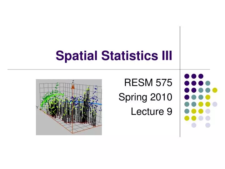
Spatial Statistics III RESM 575 Spring 2010 Lecture 9
Last time • Identifying clusters (local statistics) • Using statistics with geographic data • Analyzing geographic relationships, processes
Review • How features are distributed • What is the pattern created by the features • Where are the clusters • What are the relationships between sets of features or values • Accounting for spatial factors in our models
Today Part A. Background on Interpolation Techniques Part B. The Geostatistical Process • Explore the data • Fit a model • Perform diagnostics • Compare the models
Geostatistical Analyst of ArcGIS 9 • For advanced surface modeling • Extension of ArcGIS 9 • Tools for creating a statistically valid surface
Loading the Geostatistical Extension 1. 2. 3. 4.
Further reading • Armstrong, M. 1998. Basic Linear Geostatistics. Springer, Berlin. • Chiles, J. and Delfiner, P. 1999. Geostatistics. Modeling Spatial Uncertainty. John Wiley and Sons, New York. • Cressie, N. 1988. Spatial prediction and ordinary kriging. Mathematical Geology 20:405-421. (Erratum, Mathematical Geology 21: 493-494) • Cressie, N. 1990. The origins of kriging. Mathematical Geology 22:239-252. • Isaaks, E.H. and Srivastrava, R.M. 1989. An introduction to Applied Geostatistics. Oxford University Press, New York. • Johnston, Kevin, Jay M. Ver Hoef, Konstantin Krivoruchko, and Neil Lucas. Using ArcGis Geostatistical Analyst, 2001. Environmental System Research Institute, Redlands, CA. • Shaw, Gareth and Dennis Wheeler. Statistical Techniques in Geographical Analysis, 1994. David Fulton Publishers, London.
Part A. Background on Interpolation Techniques Deterministic methods Geostatistical methods Some important principles
Interpolating a surface • Generate the most accurate surface • Sample point data as input • Characterize the error and variability of the predicted surface
Interpolation techniques • Deterministic • Use mathematical functions for interpolation • IDW, global and local polynomial, radial basis • Geostatistical • Relies on both statistical and mathematical methods • Can be used to assess the uncertainty of the predictions NOTE: Both rely on similarity of nearby points to create the surface
Deterministic techniques • Inverse distance weighted • Global polynomial • Local polynomial • Radial bias functions
Inverse distance weighted • Reasonably accurate if the points are evenly distributed and the surface characteristics do not change across the landscape • Values of closer points are weighted more heavily than those further away
Global polynomial • Identify and model local structures and surface trends • Fit a plane between the sample points One bend = 2nd order Two bends = 3rd order Etc… Plane = first order
Local polynomial • Fitting many smaller overlapping planes
Radial basis • Captures global trends and picks up local variation (bending and stretching of surface to match all the measured values)
Geostatistical methods • Based on statistical methods not just mathematical • Include spatial autocorrelation • Provide a measure of certainty or accuracy • Kriging • Cokriging
Principals of Geostat Methods • Unlike the deterministic methods, geostatistics assumes that all values are a result of a random process with dependence • What does this mean?
Ex • Flip three coins and determine if H or T • The fourth coin will not be flipped; it will be laid down based on what the 2nd and 3rd are • Rule to lay the 4th: • if the 2nd and 3rd are tails, the fourth is the opposite of the first, if not then the 4th is same as first
How does this relate to predicting locations in an interpolation? • In coin ex, dependence rules were given • In reality, dependence rules are not known • In geostats, there are two key tasks • To uncover the dependence rules • To make predictions KEY: the predictions come from knowing the dependency rules!
Principles of Geostat Methods • Besides random process with dependence… • Stationarity • Mean stationarity • mean is constant between samples and is independent of location • Second order stationarity for covariance • covariance is the same between any two points that are at the same distance and direction apart no matter which points you choose • Intrinsic stationarity for semivariograms • variance of the difference is the same between any two points that are at the same distance and direction apart no matter which two points you choose
Kriging • In geostats, there are two key tasks • To uncover the dependence rules • To make predictions Semivariogram and covariance functions Interpolate areas
Kriging • Similar to IDW (weights surrounding values to derive a prediction) • Different in that it incorporates the spatial arrangement among the measured points (must calculate spatial autocorrelation)
Cokriging • Uses information on several variable types • Requires much more estimation (autocorrelation for each variable and cross-correlations)
Kriging process • Calculate the empirical semivariogram • Fit a model • Make a prediction
Empirical semivariogram • Tests for spatial autocorrelation (things closer are more alike) spatial modeling, structural analysis or variography Combinations of the points low on both the x and y axis have more autocorrelation Increasing dissimilarity Increasing distance
Fit a Model • Defining a line (weighted least squares) that provides the best fit through the points in the empirical semivariogram cloud • Line is considered a model quantifying the spatial autocorrelation in a model
Make a prediction • From the kriging weights for the measured values, you can calculate a prediction for the location with the unknown value.
Part B. The Geostatistical Process Explore the data Fit a model Perform diagnostics Compare the models
Why explore your data? • To make better decisions when creating a surface • To gain a better understanding of the data • Look for obvious errors in the input sample that may drastically affect the output prediction surface • Examine how the data is distributed • Look for global trends
Summarizing the Geostatistical analyst data exploration tools • Tools to examine the distribution of your data • Identify trends in the data if any • Understand the spatial autocorrelation and directional influences
Examining the distribution of data Tools Available in ArcGIS 9 Geostatistical Analyst: • Histogram • Look for normal distribution • Normal QQPlot • To find trends • Semivariogram/covariance cloud • To identify spatial autocorrelation
Histogram tool • NOTE: if mean and median are approximately • the same value, then you have reason to believe • your data is normally distributed • Interpolation results give the best results when the data is normally distributed • If skewed (lopsided) you may choose to transform the data to make it normal Make sure layer and attribute are set
Histogram tool • Important features in the histogram • Central value, spread, and symmetry Data is unimodal (one hump) and fairly symmetric, close to a normal distribution Right tail shows a small number of high ozone values
Normal QQPlot • Used to compare your distribution to a standard normal distribution • The closer your data is to the line, the more normally distributed is
Normal QQPlot The quantiles from two distributions are plotted against each other, for two identical distributions, the QQPlot will be a straight line This plot is very close to normal but departs at the selected features
Identifying global trends • Enables you to identify the presence/absence of trends in the input dataset Make sure to Set the layer and attribute
Finding trends • Each “stick” represents location and height of a data point • East/West and North/South planes • Trends are analyzed in these directions • A best fit line (polynomial) is drawn through the projected pts which models trends in the specific directions • A flat line indicates no trend N to S axis W to E axis
Interpretation of the trends • Values of ozone increase in the east to west direction • A weaker trend exists in the north to south direction • “Ozone is low at the coast, higher inland then tapers off in the mountains”
Definition of semivariogram • A function that relates dissimilarity of data points to the distance that separates them. • Its graphical representation can be used to provide a picture of the spatial correlation of data points with their neighbors
Semivariogram/covariance cloud • Examines the spatial autocorrelation between measured points • Each red dot is a pair of observations • X measures distance between the points and Y is the difference squared between the values
Semivariogram/covariance cloud interpretation • Points low on both axis represent points of higher autocorrelation (low distance between points = they are more alike) • To test areas (near areas but different) select sectors in the graph The points are primarily in LA