Download
1 / 21
210 likes | 405 Views
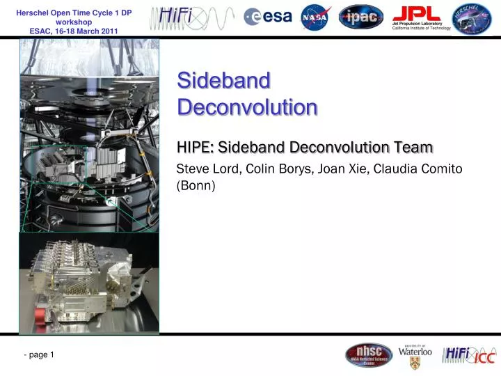
Sideband Deconvolution. HIPE: Sideband Deconvolution Team Steve Lord, Colin Borys, Joan Xie, Claudia Comito (Bonn). HIFI is a Heterodyne. Down-conversion is accomplished by forming the product: cosX cos LO = (1/2) [ cos (X - LO) + cos (X + LO) ] Like AM radio:.

E N D
Sideband Deconvolution HIPE: Sideband Deconvolution Team Steve Lord, Colin Borys, Joan Xie, Claudia Comito (Bonn)
HIFI is a Heterodyne Down-conversion is accomplished by forming the product: cosX cos LO = (1/2) [ cos (X - LO) + cos (X + LO) ] Like AM radio:
Center, colored red, is the carrier wave at 558 kHz; the two mirrored audio spectra (green) are the lower and upper sideband. AM Radio – Time plot
LO LSB + USB = DSB Lower sideband spectrum is reversed and added Two frequency scales result in the DSB result The lines may blend but they can be recovered (deconvolved) The continuum levels add (double) in the DSB The continuum slope is flattened but may be recovered (deconvolved) The noise adds in quadrature , increasing as sqrt(2)
Deconvolution Tool DemoIntro - The Problem HIFI Deconvolution tool: deconvolves HIFI’s native dual sideband observations; a crucial processing need for spectral surveys. Synthetic Spectrum T [K] 0 T[K] 200 LO Every spectrum taken with HIFI contains the upper and lower sideband data folded together. In regions rich with lines, the user needs a way to sort this out. Additionally, the upper and lower sidebands may have different gains. 800 [GHz] 850 0 T[K] 35 800.0 [GHz] 804. 816.0 [GHz] 812. Double sideband spectrum
Formulation of the Problem • Start with a guess of the answer – a model with no assumptions for the SSB spectrum – flat • "Observe it" – using knowledge of the instrument • compare the observations of the model with the real observations • compute a chi square and a delta (differential) chi-square • each model "spectral channel" was in part responsible for some of the chi square change • follow the slope of the chi square downward (it's partial derivitive w.r.t. the channel flux (and optionally the sideband gain) • new downward steps always move at right angles to previous ones in the Conjugate Gradient Method • Stop, when solution converges asymptotically, as defined by the "tolerance"
The Solution - Details With a series of LO settings, the double sidebands are marched across the band, providing a sufficient number of over-lapping “confused” observed double sideband spectra to constrain the single sideband result - I.e., the source’s true spectrum – The number of overlaps of each sideband on itself is the "Redundancy", R The iterative chi-square minimization method, the Conjugate Gradient Method finds the best single sideband solution using knowledge of the chi-square gradients. Since the problem is constrained, other methods could be used. CGM minimizes chi-square of the model residuals. Successfully used on CSO surveys and HIFI. Planned for SOFIA and ALMA (Comito & Schilke 2002), Lord, Xie, Borys...
Other Problems Deconvolving • Bad Standing Waves • Bad Baselines • "Spurs" • Gain Variations - in time or between sidebands: (this one is difficult) Some mitigation is possible • Data cleanup • Maximum Entropy added in....
10 Iterations take a few minutesConvergence after 20 iterations is typical Blue – input spectrum, Black – iterative models. Simulation c/o Claudia Comito
Successful processing – only three scans of one line SSB The gap is the range of frequencies between the sidebands - never observed DSB
CLASS90 DECON Several Routes: Ongoing testing Herschel Observations!! Synthetic spectra HIFI Simulator Level 0.5 (erased) Level 1 Bonn Simulator Level 2 (HCSS 1.2 Only) HCSS HICLASS HCSS DECON HCSS DECON CLASS90 Scripts HCSS Scripts HCSS CLASS
Deconvolution - Status and Improvement Details • Items Complete: • Conjugate Gradient Method available in HCSS v2,3,.. for all users • HCSS JAVA HIFI Deconvolution Package – up and running HCSS v2,3,4 • Interfaced and End-to-End tested with HCSS HIFI Simulator and Observations • HCSS 1,2,3… will convert Contexts (Resampling, Upper, Lower Freq.s) to Level 2 • Integrated w/HIPE – runs with scripts or GUI – viewing with spectrum explorer • Additional features Added: • Included Frequency Switching Spectral Survey Deconvolutions • Channel-by-channel weights (from Cal) included in the JAVA Software • Improving HIPE GUI with DSB Display Capabilities, DSP products, RMS vs. iteration number, SSB viewing • Importing Ghost visualization tools
HCSS Decon & XCLASS Decon Mostly in synch - but some development differences
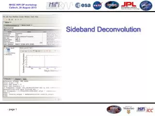
HIPE Deconvolution Task Can now turn on diagnostic mode Specify Scan Index (LO setting) Specify USB/LSB frequency axis
HIPE Deconvolution Task Interim output: DSB Input, DSB Model(iteration) for i-th LO setting, Gains(iteration) Chi-Square(iter). LO’s listed:
HIPE Deconvolution Task Metadata includes the doDeconvoluion inputs
HIPE Deconvolution Task DSB Model (iteration) vs. DSB input SSB vs. Iteration (grows!) Chi-Square vs. Iteration
HIPE Deconvolution Task Errors causing aborts are now reported with messages: e.g.: “Exceeded Maximum Iterations” Now run time